Autoregressive models
This article focuses on the first-order autoregressive model (AR(1) model), and various extensions of this. The AR(1) model is one of the simplest, yet immensely popular models for N=1 time series data. It allows you to quantify the degree to which the process you are studying is characterized by carry-over from one occasion to the next. This carry-over is captured by the autoregresssive parameter, and forms the basis of inertia research (Gottman et al., 2002; Kuppens et al., 2010; Suls et al., 1998).
You can use AR models for various research goals. For instance, you can use it to obtain parameter estimates that you consider for descriptive purposes. You can also use an AR model for forecasting, that is, to obtain predictions of the next few outcomes for an individual (for an elaborate source on this, see Hyndman & Athanasopoulos, 2021). You may also consider an AR model as the data generating mechanism. Understanding what kind of patterns the various AR models can generate is helpful in deciding whether you want to consider this as a way to analyze your data.
In this article, you find: 1) a presentation of the first-order AR model, including an interactive tool that allows you to see what kinds of temporal patterns it can generate; 2) a presentation fo the second-order AR model, including an interactive tool that allows you to see what kind of temporal patterns it can generate; 3) a presentation of the general AR model including higher-order AR processes; and 4) a discussion of how this model is related to other models for N=1 ILD.
1 First-order autoregressive model: AR(1) model
Suppose you have a time series consisting of univariate measurements of the variable \(y\), obtained at equal time intervals. The observation at occasion \(t\) is denoted as \(y_t\). If this time series is a first-order AR model, this implies that each observation \(y_t\) can be partly predicted by the observation immediately preceding it \(y_{t-1}\), but that there is also an unpredictable part \(\epsilon_t\). There are various ways in which you can represent an AR(1) model.
First, you can visualize it as in Figure 2.

Second, you can represent an AR(1) model with the equation
\[y_t = c + \phi_1 y_{t-1} + \epsilon_t ,\] where: \(c\) is a constant that is referred to as the intercept; \(\phi_1\) is the AR parameter, also referred to as carry-over or inertia; and \(\epsilon_t\) is the unpredictable part that is referred to as the innovation, residual, random shock, perturbation, (dynamic) error, or disturbance. The innovations are independently and identically distributed, and typically it is assumed they come from a normal distribution with a mean of zero and variance \(\sigma^2_\epsilon\).
Below, you find a more elaborate explanation of the various parameters of the AR(1) model, as well as an explanation of the constraint that is needed to ensure the process is stationary, and why this is important. There is also an interactive tool that allows you to investigate the role that each parameter plays in the kind of temporal patterns that an AR(1) process can generate.
1.1 The intercept \(c\) versus the mean \(\mu\) in an AR(1) process
As in any regression, the intercept represents the predicted value for the outcome (here: \(y_t\)) when the predictor (here: \(y_{t-1}\)) has a value of zero. While this may be of interest when \(y\) can take on the value zero, it may be rather uninformative if this never happens and especially if this is not even possible given the scale of \(y\).
Ove obtained daily measures of happiness from himself over 100 days, using a scale from 1 to 10. He makes two plots of this, as shown below. The plot on the left shows Ove’s happiness plotted against time. The blue dotted line represents his mean over the 100 occasions. The plot on the right shows Ove’s happiness at occasion \(t\) plotted against his happiness at occasion \(t-1\). You can think of this as his happiness today, plotted against his happiness yesterday. Again the dotted blue lines represent the mean of Ove’s happiness across the 100 days.
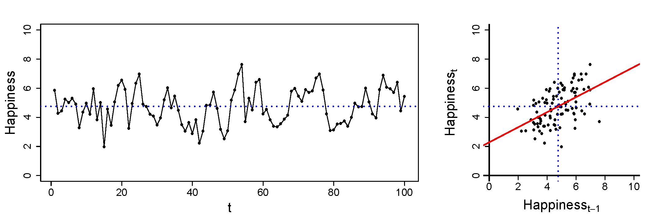
The red line in the plot on the right represents the relation between Ove’s happiness today and his happiness yesterday. If Ove uses an AR(1) model for these data, the AR parameter \(\phi_1\) that he would obtain would be (about) equal to the slope of this red line. Furthermore, the intercept \(c\) in that model would be (about) the value at which the line crosses the y-axis.
When thinking about this, it becomes clear to Ove that the intercept \(c\) is really not of interest to him: As the happiness was measured on a scale that runs from 1 to 10, it is impossible to obtain a score of 0. Hence. knowing what value to expect today, if he had scored 0 on happiness yesterday, is not something that is meaningful from a substantive point of view.
If the current data were obtained with a scale that runs from 0 to 10, the intercept \(c\) would still not have been very interesting to Ove, simply because he never scored zero on happiness.
Ove is more interested in knowing what his mean happiness is; this is represented by the dotted blue line, but it is not a parameter that Ove obtains when he estimates the AR(1) model.
Often, it can be considered more interesting to obtain the mean of \(y\), instead of the intercept; the mean represents the central tendency of a person, and is also described as a person’s equilibrium or baseline to which they return if there are no external influences (i.e., innovations). You can rewriting the AR(1) process as
\[y_t = \mu + \phi_1 (y_{t-1}-\mu) + \epsilon_t ,\] where \(\mu\) represents the mean of \(y\).
This mean can be related to the intercept through a well-known expression from the time series literature (e.g., Hamilton, 1994), that is,
\[\mu = \frac{c}{1-\phi_1}\] and thus
\[c = (1-\phi_1) \mu .\] This shows that the intercept \(c\) is equal to the mean \(\mu\) if either the mean is zero (i.e., \(c=\mu=0\)), or if the AR parameter is zero (i.e., \(\phi_1=0\)). In all other scenarios, the mean and intercept differ.
You can read more about the difference between \(\mu\) and \(c\) in the article about the two formulations of an AR model.
1.2 The variance of \(y\) versus the variance of \(\epsilon\)
The variance of an AR(1) process can be expressed as a function of the variance of the innovations, through
\[ \sigma_y^2 = \frac{\sigma_{\epsilon}^2}{1-\phi_1^2} .\]
This shows that if \(\phi_1=0\), the variance of \(y\) is the same as the variance of \(\epsilon\) (i.e, \(\sigma_y^2=\sigma_{\epsilon}^2\)). But if \(\phi_1 \neq 0\), the variance of \(y\) will be larger than that of \(\epsilon\). From a substantive point of view, this makes sense, because \(\epsilon\) is the part of \(y\) that cannot be predicted by the autoregression in \(y\); hence, \(\sigma_{\epsilon}^2\) is the variance in \(y\) that cannot be accounted for by the AR part of the model, and it is thus necessarily smaller (or equal to) the variance of \(y\).
The expression above also implies that
\[ \sigma_{\epsilon}^2 = (1-\phi_1^2) \sigma_y^2 .\]
Hence, if you know two of the three parameters \(\phi_1\), \(\sigma_{\epsilon}^2\), and \(\sigma_{y}^2\), you also know the third.
1.3 Interpretation of the autoregressive parameter \(\phi_1\)
The autoregressive parameter can be thought of as a slope: When you consider \(y_{t-1}\) as the predictor and \(y_t\) as the outcome, the steepness of the slope will be determined by \(\phi_1\). This is illustrated in Figure 3.

Another way to think about the autoregressive parameter in an AR(1) process is that it quantifies the degree to which there is carry-over from \(y_{t-1}\) into \(y_t\). When it is 0, there is no carry-over from one occasion to the next; the closer the autoregression is to 1, the larger the degree of carry-over.
Because of this property, the autoregressive parameter has also been referred to as inertia (Gottman et al., 2002; Suls et al., 1998) or regulatory weakness (Haan-Rietdijk et al., 2016; Kuppens et al., 2010) in the psychological literature: It captures the degree to which a person tends to get stuck in a certain state for longer periods of time.
This is clearly visible when considering the time series plots in the left of Figure 3: The top one is based on having \(\phi_1=0.3\) and shows more randomness in the fluctuations over time, whereas the bottom one is based on \(\phi_1=0.9\) and is characterized by less random fluctuations over time.
Although not so common in psychological research, it is also possible that the autoregressive parameter is negative.
Mike is studying daily alcohol consumption in a person who is identified as a heavy drinker. He decides to analyze the daily diary data with an AR(1) model and expects to find a positive autoregressive parameter; that parameter would indicate that days on which the person drank a lot are often followed by more days on which they drink a lot, while days on which they drank less than usual tend to be followed by more days on which they drink less.
However, after running the analysis, Mike obtains a negative autoregressive parameter. After thinking about what such a result implies, he comes to the conclusion that this can be interpreted as follows: When this person drank a lot on one day, they are less likely to drink a lot the following day, perhaps because they are hung-over; but if they drank less than usual on a particular day, they become more likely to drink heavily the next day. Hence, the negative autoregressive parameter can be thought of as reflecting a form of compensating behavior.
From the perspective of your research goal, the interpretation of the autoregressive parameter may differ depending on whether your research goal is description, prediction or causation. When your goal is description, you may simply use the autoregressive parameter as a quantification of temporal (or sequential) dependencies in your data. When your goal is prediction, the autoregressive parameter may be used to make forecasts for the next few occasions. When your goal is to study causation, the model may be viewed as the data generating mechanism, where the autoregressive parameter is not just a feature that can be obtained from the data, but it forms an actual force that shapes the process.
What is also useful to know when you want to interpret the autoregressive parameter of an AR(1) model, is that you can think of this parameter as already being standardized: Since the predictor \(y_{t-1}\) and the outcome \(y_t\) are the same variable with the same variance \(\sigma_y^2\), standardizing \(\phi_1\) does not change its value. Moreover, \(\phi_1\) of an AR(1) model it is equal to the [autocorrelation] at lag 1.
1.4 Stationarity of an AR(1) process
Autoregressive processes are by definition stationary, which means that their mean, variance, and other properties are invariant (i.e., constant) over time. To ensure that the process that is expressed above is stationary, the autoregressive parameter needs to lie between \(-1\) and \(1\), that is
\[ -1 < \phi_1 < 1\]
or
\[ |\phi_1| <1 \] When the autoregressive parameter is equal to 1, the process is not an AR(1) model any more, but is known as a [random walk]. Such a process is non-stationary, and is characterized by very different behavior over time than an autoregressive process. Hence, the point here is not that is it impossible for the autoregressive parameter to be equal to 1 or larger (or equal to \(-1\) or even smaller); this is possible, but this is not an autoregressive process then.
In practice, the autoregressive parameter may be smaller than 1 but perhaps quite close to it; in that case it may be difficult to determine whether the process is stationary (i.e., an autoregressive process), or that it is not stationary (e.g., a random walk). There are specific [tests] that you can use to investigate whether your time series is stationary or not.
1.5 Interactive tool of an AR(1) process
Below is an interactive tool that allows you to obtain an intuition for what kinds of temporal patterns an AR(1) model can generate. Specifically, it allows you to change the number of occasions and the values of the mean, variance, and autoregressive parameters of an AR(1) model, so that you can see how each of them plays a role in the process.
#| '!! shinylive warning !!': |
#| shinylive does not work in self-contained HTML documents.
#| Please set `embed-resources: false` in your metadata.
#| standalone: true
#| viewerHeight: 410
library(shiny)
library(bslib)
## file: app.R
library(shiny)
library(bslib)
library(ggplot2)
library(patchwork)
simulateData <- function(n, mu, sigma, phi) {
burnin <- 100
burnin_t <- n + burnin
innov_var <- sigma * (1 - phi ^ 2)
e <- rnorm(burnin_t, sd = sqrt(innov_var))
y <- numeric(burnin_t)
for (t in 2:burnin_t) {
y[t] <- mu + phi * (y[t - 1] - mu) + e[t]
}
y <- y[(burnin + 1):burnin_t]
dat <- data.frame(y = y, t = 1:n)
return(dat)
}
plotTimeSeries <- function(dat, plot_widths = c(2, 5, 1)) {
x_breaks <- pretty(1:nrow(dat))
y_breaks <- pretty(dat$y)
y_lim <- c(min(y_breaks), max(y_breaks))
axis_line_width <- 0.3
dat$y_lag <- c(NA, dat$y[-length(dat$y)])
coryy <- round(cor(dat$y, dat$y_lag, use = "complete.obs"), 3)
meany <- mean(dat$y)
lm1 <- lm(y ~ y_lag, dat)
ys1 <- cbind(1, c(min(y_breaks), max(y_breaks))) %*% coef(lm1)
p_ss <- ggplot(dat, aes(x = y_lag, y = y)) +
geom_segment(aes(x = min(y_breaks), xend = max(y_breaks),
y = ys1[1], yend = ys1[2]),
linewidth = 0.3, colour = "gray") +
geom_point(size = 2, shape = 21, fill = "white") +
scale_y_continuous(breaks = y_breaks) +
scale_x_continuous(breaks = y_breaks) +
coord_cartesian(ylim = y_lim, xlim = y_lim) +
theme_void() +
labs(x = bquote(y[t-1]), y = bquote(y[t])) +
theme(text = element_text(family = "sans", size = 16),
axis.text = element_text(margin = margin(5, 5, 5, 5)),
axis.title = element_text(margin = margin(5, 5, 5, 5)),
axis.ticks = element_line(lineend = "butt",
linewidth = axis_line_width),
axis.ticks.length = unit(2.5, "pt"),
panel.spacing = unit(5, units = "pt"),
plot.margin = margin(0, 5, 0, 0),
legend.position = "none") +
geom_segment(x = -Inf, xend = -Inf, y = y_breaks[1],
yend = y_breaks[length(y_breaks)],
linewidth = axis_line_width, lineend = "square") +
geom_segment(y = -Inf, yend = -Inf, x = y_breaks[1],
xend = y_breaks[length(y_breaks)],
linewidth = axis_line_width, lineend = "square") +
annotate("text", x = -Inf, y = Inf, hjust = -0.2, vjust = 2,
label = bquote(hat(rho)[1]~"="~.(coryy)), size = 5)
p_ts <- ggplot(dat) +
geom_segment(x = x_breaks[1], xend = max(x_breaks), y = meany, yend = meany,
linewidth = 0.3, colour = "gray") +
geom_line(aes(x = t, y = y)) +
geom_point(aes(x = t, y = y), size = 2, shape = 21, fill = "white") +
scale_y_continuous(breaks = y_breaks) +
scale_x_continuous(breaks = x_breaks) +
coord_cartesian(ylim = y_lim, xlim = c(min(x_breaks), max(x_breaks))) +
theme_void() +
labs(x = "t") +
theme(text = element_text(family = "sans", size = 16),
axis.text.x = element_text(margin = margin(5, 5, 5, 5)),
axis.title.x = element_text(margin = margin(5, 5, 5, 5)),
axis.ticks = element_line(lineend = "butt",
linewidth = axis_line_width),
axis.ticks.length = unit(2.5, "pt"),
panel.spacing = unit(5, units = "pt"),
plot.margin = margin(0, 5, 0, 0),
legend.position = "none") +
geom_segment(x = -Inf, xend = -Inf, y = y_breaks[1], yend = max(y_breaks),
linewidth = axis_line_width, lineend = "square") +
geom_segment(y = -Inf, yend = -Inf, x = x_breaks[1], xend = max(x_breaks),
linewidth = axis_line_width, lineend = "square")
p_hist <- ggplot(dat) +
geom_histogram(aes(y = y, x = ..density..), fill = "gray", colour = "black") +
geom_density(aes(y = y)) +
geom_hline(yintercept = meany, colour = "gray", linewidth = 0.5) +
scale_y_continuous(breaks = y_breaks) +
scale_x_continuous(breaks = x_breaks) +
coord_cartesian(ylim = y_lim) +
theme_void() +
labs(x = "", y = "") +
theme(text = element_text(family = "sans", size = 16),
axis.title = element_text(margin = margin(5, 5, 5, 5)),
panel.spacing = unit(5, units = "pt"),
plot.margin = margin(0, 5, 0, 0))
p <- p_ss + p_ts + p_hist + plot_layout(widths = plot_widths)
return(p)
}
ui <- fluidPage(
fluidRow(
column(3,
numericInput("n", label = h4("Number of occasions T"), value = 100,
min = 10, max = 1e5, step = 10)
),
column(3,
numericInput("mean", label = HTML("<h4>Mean μ</h4>"), value = 0, step = 1)
),
column(3,
numericInput("var", label = HTML("<h4>Variance σ<sup>2</sup><sub style='position: relative; left: -0.4em;'>y</sub></h4>"),
value = 1, min = 0, max = 100, step = 1)
),
column(3,
sliderInput("autoregression", label = HTML("<h4>Autoregression \U03D5<sub>1</sub></h4>"), min = -0.999,
max = 0.999, value = 0.3, step = 0.05)
)
),
actionButton("refresh", "Refresh"),
plotOutput(outputId = "main_plot", height = "250px"),
)
server <- function(input, output) {
dat <- reactive({
input$refresh # include to make it reactive to the button
simulateData(input$n, input$mean, input$var, input$autoregression)
})
output$main_plot <- renderPlot({
plotTimeSeries(dat())
})
}
shinyApp(ui = ui, server = server)
The tool shows three visualizations of the data that are generated from an AR(1) model with the specified parameter values and number of occasions. The left figure is an autocorrelation scatter plot of \(y\) at occasion \(t\) against \(y\) at the previous occasion \(t-1\), with the lag-1 autocorrelation \(\hat{\rho}_1\) of the generated data and a straight line indicating the linear relationship. The middle figure is a time series plot of \(y\) against time, where the horizontal grey line indicates the observed mean of the series. Finally, the right figure shows the distribution as a histogram and a density line, again with a horizontal grey line indicating the observed mean. The refresh button allows you to generate a new data set with the same specifications.
2 Second-order autoregressive model: AR(2) model
The AR(1) model presented above can be extended to a higher-order autoregressive process. For instance, in Figure 4 you see a second-order version, known as an AR(2) model.

The AR(2) model can be expressed as
\[y_t = c + \phi_1 y_{t-1} + \phi_2 y_{t-2} + \epsilon_t ,\] showing that the current score \(y_t\) is partly predicted by the scores preceding it, that is \(y_{t-1}\) and \(y_{t-2}\), and part of it is not predictable and captured by the innovation \(\epsilon_t\).
From the graphical representation of the AR(2) model you can see that \(y_{t-2}\) has both a direct and an indirect effect on \(y_t\): The direct effect is captured by \(\phi_2\), whereas the indirect effect is mediated by \(y_{t-1}\) and equals \(\phi_1^2\).
In this section you find a more elaborate explanation of the various parameters of the AR(2) model, as well as an an explanation of the constraints that are needed to ensure an AR(2) process is stationary. There is also an interactive tool that allows you to investigate the role that each parameter plays in the kind of temporal patterns that an AR(2) process can generate.
2.1 The intercept \(c\) versus the mean \(\mu\) in an AR(2) process
As in the case of the AR(1) model, in the AR(2) model the intercept \(c\) may not be very meaningful from a substantive point of view. Instead of using the expression with the uncentered lagged predictors, you can re-express the AR(2) model using centered predictors, that is
\[y_t = \mu + \phi_1 (y_{t-1}-\mu) + \phi_2 (y_{t-2}-\mu) + \epsilon_t ,\] where \(\mu\) is the mean, which can also be thought of as the equilibrium or baseline of a person.
In an AR(2), the mean and the intercept are related through
\[ \mu = \frac{c}{1-\phi_1 -\phi_2} \] and thus
\[ c = (1-\phi_1 -\phi_2) \mu .\]
2.2 The variance of \(y\) versus the variance of \(\epsilon\)
The variance of an AR(2) process is already a rather complex function of the variance of the innovations and the autoregressive parameters, that is
\[ \sigma_y^2 = \frac{(1-\phi_2)\sigma_{\epsilon}^2}{(1+\phi_2)(1-\phi_1-\phi_2)(1+\phi_1-\phi_2)} .\]
The variance of an AR(2) model is the same as the variance of the innovations \(\epsilon\) if the autoregressive parameters are both zero. Moreover, when the autoregressive parameters are non-zero, the variance of \(y\) will be larger than that of \(\epsilon\).
2.3 Interpretation of the autoregressive parameters \(\phi_1\) and \(\phi_2\)
The autoregressive parameters in an AR(2) model are somewhat harder to interpret than the single autoregressive parameter in an AR(1) model. From a predictive point of view you may find that an AR(2) model provides better forecasts, but it may also be the case that out-of-sample performance of you forecasts is better when you use a simpler AR(1) model.
If we think of it in terms of a data generating mechanism of for instance daily stress levels, the AR(2) model implies that today’s stress \(y_t\) is not only determined by carry-over from yesterday’s stress \(y_{t-1}\), but that it also is directly affected by the stress of the day before yesterday \(y_{t-2}\). You may have noticed that in an AR(1) model, there is also a relation between today’s stress \(y_t\) and the day before yesterday’s stress \(y_{t-2}\), but this is fully mediated by yesterday’s stress \(y_{t-1}\); once you condition on yesterday’s stress \(y_{t-1}\), there is no additional information in the day before yesterday’s stress \(y_{t-2}\) that is related to today’s stress \(y_t\).
As was the case in the AR(1) model, the parameters of the AR(2) model can be thought of as already standardized. However, their relation to the underlying autocorrelations is more complicated than for an AR(1) process. Specifically, \(\phi_2\) can be thought of as the [partial autocorrelation] at lag two.
2.4 Stationarity of an AR(2) process
The stationarity conditions for an AR(2) process are more involved than those for an AR(1) process. Specifically, the following three conditions must be met:
\(-1 < \phi_2 < 1\)
\((\phi_2 + \phi_1) < 1\)
\((\phi_2 - \phi_1) < 1\)
While the first condition is similar to the condition for \(\phi_1\) in an AR(1) process, the other two conditions are about the specific combination of parameter values. The three conditions can be visualized together by showing the area in the \(\phi_1\) and \(\phi_2\) space that results in a stationary AR(2) process; this is done in Figure 5.

When the two parameter values fall inside the blue triangle, the process is stationary, and it can thus be considered an autoregressive process. When the parameters fall outside the blue triangle, the process is not stationary, and hence it is not an autoregressive process.
The red dashed line that is included in Figure 5 divides the processes into two categories: a) below the red dashed curve, the process is oscillating; b) above the red dashed curve, the process is non-oscillating. You can try this out for stationary AR(2) processes with the interactive tool presented above. For instance, if you set \(\phi_1=0\) and \(\phi_2 = -0.8\), you obtain an oscillating process. In contrast, when you change \(\phi_2\) from -0.8 to 0.8, you have a non-oscillating process.
Mike has obtained data from a second person who is identified as a heavy drinker, and wonders whether these two persons are characterized by similar patterns in their drinking behavior, such that they can be modeled with a similar model. To see what kind of temporal dependencies there are in the data, he plots the autocorrelation functions and the partial autocorrelation functions of both persons side by side, as shown below.

Mike notices that, while they both tend to alternate between positive and negative autocorrelations as the lag size increases, the patterns are quite different across the two persons. Person 1 alternates rapidly (i.e., every other lag has changes sign), and the decay in (absolute) values is exponential, which is typical of an AR(1) process with a negative autoregressive parameter. In contrast, the sign of the autocorrelations of person 2 do not change sign as rapidly when increasing the lag, but their values go to zero much quicker.
When considering the partial autocorrelation, Mike notices that for person 1, all the partial autocorrelations from lag 2 onward seem to be zero; this is typical of an AR(1) process. In contrast, for person 2, there is a large partial autocorrelation at lag 2, and after that the partial autocorrelations are about zero. Mike knows this is typical of an AR(2) process.
He can further investigate this difference by fitting both an AR(1) and an AR(2) model to the data of both individuals, and do a model comparison for each person (e.g., using a log likelihood ratio test or using another model comparison metric).
To determine whether your process is stationary or not, you can make use of specific [tests].
2.5 Interactive tool of an AR(2) process
Below is an interactive tool that allows you to obtain an intuition for what kinds of temporal patterns an AR(2) model can generate. Specifically, it allows you to change the number of occasions and the values of the mean, variance, and autoregressive parameters of an AR(2) model, so that you can see how each of them plays a role in the process.
#| '!! shinylive warning !!': |
#| shinylive does not work in self-contained HTML documents.
#| Please set `embed-resources: false` in your metadata.
#| standalone: true
#| viewerHeight: 410
library(shiny)
library(bslib)
## file: app.R
library(shiny)
library(bslib)
library(ggplot2)
library(patchwork)
simulateData <- function(n, mu, sigma, phi1, phi2) {
burnin <- 100
burnin_t <- n + burnin
innov_var <- sigma * (1 + phi2) * (1 - phi1 - phi2) * (1 + phi1 - phi2) / (1 - phi2)
e <- rnorm(burnin_t, sd = sqrt(innov_var))
y <- numeric(burnin_t)
for (t in 3:burnin_t) {
y[t] <- mu + phi1 * (y[t - 1] - mu) + phi2 * (y[t - 2] - mu) + e[t]
}
y <- y[(burnin + 1):burnin_t]
dat <- data.frame(y = y, t = 1:n)
return(dat)
}
nDec <- function(x) {
sapply(x, function(y) nchar(sub("^-?\\d*\\.?", "", format(y, scientific = F))))
}
plotTimeSeries <- function(dat, plot_widths = c(3, 3, 6, 1)) {
n <- nrow(dat)
x_breaks <- pretty(1:n)
y_breaks <- pretty(dat$y)
y_lim <- c(min(y_breaks), max(y_breaks))
axis_line_width <- 0.3
dat$y_lag1 <- c(NA, dat$y[-n])
dat$y_lag2 <- c(NA, NA, dat$y[-c(n, n-1)])
coryy1 <- round(cor(dat$y, dat$y_lag1, use = "complete.obs"), 3)
coryy2 <- round(cor(dat$y, dat$y_lag2, use = "complete.obs"), 3)
meany <- mean(dat$y)
lm1 <- lm(y ~ y_lag1, dat)
ys1 <- cbind(1, c(min(y_breaks), max(y_breaks))) %*% coef(lm1)
lm2 <- lm(y ~ y_lag2, dat)
ys2 <- cbind(1, c(min(y_breaks), max(y_breaks))) %*% coef(lm2)
angle_x <- ifelse(max(nDec(y_breaks)) > 0, 30, 0)
p_ss1 <- ggplot(dat, aes(x = y_lag1, y = y)) +
geom_segment(aes(x = min(y_breaks), xend = max(y_breaks),
y = ys1[1], yend = ys1[2]),
linewidth = 0.3, colour = "gray") +
geom_point(size = 2, shape = 21, fill = "white") +
scale_y_continuous(breaks = y_breaks) +
scale_x_continuous(breaks = y_breaks) +
coord_cartesian(ylim = y_lim, xlim = y_lim) +
theme_void() +
labs(x = bquote(y[t-1]), y = bquote(y[t])) +
theme(text = element_text(family = "sans", size = 16),
axis.text = element_text(margin = margin(5, 5, 5, 5)),
axis.text.x = element_text(angle = angle_x),
axis.title = element_text(margin = margin(5, 5, 5, 0)),
axis.ticks = element_line(lineend = "butt",
linewidth = axis_line_width),
axis.ticks.length = unit(2.5, "pt"),
panel.spacing = unit(5, units = "pt"),
plot.margin = margin(0, 5, 0, 0),
legend.position = "none") +
geom_segment(x = -Inf, xend = -Inf, y = y_breaks[1],
yend = y_breaks[length(y_breaks)],
linewidth = axis_line_width, lineend = "square") +
geom_segment(y = -Inf, yend = -Inf, x = y_breaks[1],
xend = y_breaks[length(y_breaks)],
linewidth = axis_line_width, lineend = "square") +
annotate("text", x = -Inf, y = Inf, hjust = -0.2, vjust = 2,
label = bquote(hat(rho)[1]~"="~.(coryy1)), size = 5)
p_ss2 <- ggplot(dat, aes(x = y_lag2, y = y)) +
geom_segment(aes(x = min(y_breaks), xend = max(y_breaks),
y = ys2[1], yend = ys2[2]),
linewidth = 0.3, colour = "gray") +
geom_point(size = 2, shape = 21, fill = "white") +
scale_y_continuous(breaks = y_breaks) +
scale_x_continuous(breaks = y_breaks) +
coord_cartesian(ylim = y_lim, xlim = y_lim) +
theme_void() +
labs(x = bquote(y[t-2])) +
theme(text = element_text(family = "sans", size = 16),
axis.text.x = element_text(margin = margin(5, 5, 5, 5), angle = angle_x),
axis.title.x = element_text(margin = margin(5, 5, 5, 5)),
axis.ticks = element_line(lineend = "butt",
linewidth = axis_line_width),
axis.ticks.length = unit(2.5, "pt"),
panel.spacing = unit(5, units = "pt"),
plot.margin = margin(0, 5, 0, 0),
legend.position = "none") +
geom_segment(x = -Inf, xend = -Inf, y = y_breaks[1],
yend = y_breaks[length(y_breaks)],
linewidth = axis_line_width, lineend = "square") +
geom_segment(y = -Inf, yend = -Inf, x = y_breaks[1],
xend = y_breaks[length(y_breaks)],
linewidth = axis_line_width, lineend = "square") +
annotate("text", x = -Inf, y = Inf, hjust = -0.2, vjust = 2,
label = bquote(hat(rho)[2]~"="~.(coryy2)), size = 5)
p_ts <- ggplot(dat) +
geom_segment(x = x_breaks[1], xend = max(x_breaks), y = meany, yend = meany,
linewidth = 0.3, colour = "gray") +
geom_line(aes(x = t, y = y)) +
geom_point(aes(x = t, y = y), size = 2, shape = 21, fill = "white") +
scale_y_continuous(breaks = y_breaks) +
scale_x_continuous(breaks = x_breaks) +
coord_cartesian(ylim = y_lim, xlim = c(min(x_breaks), max(x_breaks))) +
theme_void() +
labs(x = "t") +
theme(text = element_text(family = "sans", size = 16),
axis.text.x = element_text(margin = margin(5, 5, 5, 5)),
axis.title.x = element_text(margin = margin(5, 5, 5, 5)),
axis.ticks = element_line(lineend = "butt",
linewidth = axis_line_width),
axis.ticks.length = unit(2.5, "pt"),
panel.spacing = unit(5, units = "pt"),
plot.margin = margin(0, 5, 0, 0),
legend.position = "none") +
geom_segment(x = -Inf, xend = -Inf, y = y_breaks[1], yend = max(y_breaks),
linewidth = axis_line_width, lineend = "square") +
geom_segment(y = -Inf, yend = -Inf, x = x_breaks[1], xend = max(x_breaks),
linewidth = axis_line_width, lineend = "square")
p_hist <- ggplot(dat) +
geom_histogram(aes(y = y, x = ..density..), fill = "gray", colour = "black") +
geom_density(aes(y = y)) +
geom_hline(yintercept = meany, colour = "gray", linewidth = 0.5) +
scale_y_continuous(breaks = y_breaks) +
scale_x_continuous(breaks = x_breaks) +
coord_cartesian(ylim = y_lim) +
theme_void() +
labs(x = "", y = "") +
theme(text = element_text(family = "sans", size = 16),
axis.title = element_text(margin = margin(5, 5, 5, 5)),
panel.spacing = unit(5, units = "pt"),
plot.margin = margin(0, 5, 0, 0))
p <- p_ss1 + p_ss2 + p_ts + p_hist + plot_layout(widths = plot_widths)
return(p)
}
ui <- fluidPage(
fluidRow(
column(2,
numericInput("n", label = h4("# occasions T"), value = 100,
min = 10, max = 1e5, step = 10)
),
column(2,
numericInput("mean", label = HTML("<h4>Mean μ</h4>"), value = 0, step = 1)
),
column(2,
numericInput("var", label = HTML("<h4>Variance σ<sup>2</sup><sub style='position: relative; left: -0.4em;'>y</sub></h4>"),
value = 1, min = 0, max = 100, step = 1)
),
column(3,
sliderInput("autoregression", label = HTML("<h4>Autoregression \U03D5<sub>1</sub></h4>"), min = -2,
max = 2, value = 0.3, step = 0.05)
),
column(3,
sliderInput("autoregression2", label = HTML("<h4>Autoregression \U03D5<sub>2</sub></h4>"), min = -1,
max = 1, value = 0.3, step = 0.05)
)
),
actionButton("refresh", "Refresh"),
plotOutput(outputId = "main_plot", height = "250px"),
)
server <- function(input, output) {
dat <- reactive({
validate(
need((input$autoregression2 + input$autoregression) < 1 & (input$autoregression2 - input$autoregression) < 1,
"The specified autoregressive parameter values do not satisfy stationary conditions.")
)
input$refresh # include to make it reactive to the button
simulateData(input$n, input$mean, input$var,
input$autoregression, input$autoregression2)
})
output$main_plot <- renderPlot({
plotTimeSeries(dat())
})
}
shinyApp(ui = ui, server = server)
The tool shows four visualizations of data that are generated from an AR(2) model with the specified parameter values and number of occasions. The first figure is an autocorrelation scatter plot of \(y\) at occasion \(t\) against \(y\) at the previous occasion \(t-1\), with the lag-1 autocorrelation \(\hat{\rho}_1\) of the generated data and a straight line indicating the linear relationship. The second figure is an autocorrelation scatter plot of \(y\) at occasion \(t\) against \(y\) two occasions ago \(t-2\), with the lag-2 autocorrelation \(\hat{\rho}_2\) of the generated data and a straight line indicating the linear relationship. Note that the autocorrelations are not the same as the autoregressive parameters, as they do not control for other lags. Furthermore, as explained in the previous section (-Section 2.4), some combinations of \(\phi_1\) and \(\phi_2\) imply a non-stationary process in which case the tool will show a message and not generate data. The third figure is a time series plot of \(y\) against time, where the horizontal grey line indicates the observed mean of the series. Finally, the right figure shows the distribution as a histogram and a density line, again with a horizontal grey line indicating the observed mean. The refresh button allows you to generate a new data set with the same specifications.
3 Higher order autoregressive models: AR(p) model
More generally, an autoregressive model of order \(p\) can be expressed as
\[y_t = c + \phi_1 y_{t-1} + \phi_2 y_{t-2} + \dots + \phi_p y_{t-p} + \epsilon_t ,\] Alternatively this can be expressed using the summation symbol as
\[y_t = c + \sum_{j=1}^p \phi_j y_{t-j} + \epsilon_t .\] In this section, you can read about the relations between the intercept \(c\) and the mean \(\mu\) in an AR(p) model, and about stationarity in the context of an AR(p) process. Although there is an analytical expression that shows how the variance of an AR(p) model can be written as a function fo the variance of the innovations and the autoregressive parameters, this expression requires the use of the backshift operator (Hamilton, 1994); this is beyond the scope of MATILDA.
3.1 The intercept \(c\) verus the mean \(\mu\) in an AR(p) process
This general model can also be re-expressed such that we have the mean rather than the intercept; this requires using the mean-centered lagged versions of the outcome on the right-hand side, that is
\[y_t = \mu + \sum_{j=1}^p \phi_j (y_{t-j}-\mu) + \epsilon_t .\]
The mean and the intercept of an AR(p) are related through
\[\mu = \frac{c}{1 - \phi_1 - \phi_2 - \dots - \phi_p} ,\] and thus
\[ c = (1 - \phi_1 - \phi_2 - \dots - \phi_p) \mu .\]
3.2 Stationarity of an AR(p) process
The conditions for stationarity of an AR(p) process are rather complex, and cannot be expressed easily. In general, it can be said that the roots of the lag polynomial must lie outside the unit root circle (cf. Hamilton, 1994); but to understand this, you need to dive into what a lag polynomial is, what it roots are, and what the unit root circle is. This is beyond the scope of MATILDA.
From a more pragmatic point of view, you can make use of existing [stationarity tests] to see whether an observed time series shows signs of non-stationarity, include (but not limited to) non-stationarity due to not meeting the criteria needed for a stationary AR(p) process.
4 Relations with other models
There are many ways to connect the models covered in this article to other models for ILD (Hamaker & Dolan, 2009). The autoregressive models for N=1 ILD can be seen as special cases of the more general class of [autoregressive moving average (ARMA) models]. There are also multivariate extensions of this, which are known as [vector autoregressive (VAR) models] and [vector autoregressive moving average (VARMA) models].
Other extensions consist of including an exogenous variable, that can be concurrent, known as the [ARX model], or lagged. A common way to extend these models is by including time \(t\) as a predictor, to account for a deterministic trend over time; this can be further extended by including also the square of time \(t^2\), and possibly even higher-order polynomials, allowing for more diverse deterministic trajectories over time.
There are also extensions of the autoregressive model that allow the parameters to vary over time; these are referred to as [time-varying autoregressive (TV-AR) models]. Closely related are [regime-switching models], and [threshold autoregressive (TAR) models].
The autoregressive models fall within the broad category of [discrete time] models; they have a [continuous time] equivalent based on differential equations.
For many–but not all–of these extensions and alternatives, multilevel versions have been developed to accommodate N>1 ILD.
5 Think more about
An autoregressive model–like many other time series models–is based on having equal time intervals between your measurements occasions. This is a requirement that is easily (approximately) met in [daily diary studies], where measurements are obtained once per day in the evening. It is also easily met in studies that involve [physiological measurements], or [expert ratings] of behaviors based on video recordings; such measurements tend to be regularly spaced in time, for instance, every second or every five seconds.
But there are also measurement designs in which this requirement is by definition–and even on purpose–violated. For instance, in [experience sampling] or [ecological momentary assessments] the observations are obtained by measuring at irregular time intervals throughout the day, to avoid participants anticipating the next measurement occasion. Also, [event contingency] measurements, which require measurements to occur after a particular event (i.e., a social interaction or a panic attack), are likely to have wildly varying time intervals.
Although there is thus a discrepancy between the basis of autoregressive models and many of the types of data in ILD research, there are various ways to tackle this (e.g., Haan-Rietdijk et al., 2017). You can read more about this in the article on [dealing with irregular time intervals].
Another aspect to keep in mind is that autoregressive models are stationary, but that the trajectories they generate not always look stationary. That is, when there is a large displacement in an autoregressive process, this can result in a gradual increasing or decreasing trajectory over time back towards the long-run mean \(\mu\) that characterizes the process. You can try this out with the displacement tool.
To estimate the parameters of an autoregressive model, there are various options. Historically, the Yule-Walker equations were often used for this, but nowadays estimation typically relies on some kind of Kalman filter procedure. You can read more about this in the article about [estimation] of time series models.
6 Takeaway
The univariate stationary autoregressive model is often used as the basis for analyzing time series data. The most important feature of an autoregressive process is its order \(p\), which indicates how many previous occasions provide unique information to predict the current score: When the order is 1, only the score at lag 1 (i.e., \(y_{t-1}\)) contains unique information; when the order is 2, both \(y_{t-1}\) and \(y_{t-2}\) contain unique information about \(y_t\); when the order is \(p\), then \(y_{t-1}\) up to \(y_{t-p}\) contain unique information.
The order of an autoregressive process, and the actual values of the autoregressive parameter(s) determine what kind of behaviors a process can generate over time. You can try this out for an AR(1) and an AR(2) process with the interactive tools that are included above. The larger \(p\) is, the more complicated and diverse the patterns are that can be generated.
The autoregressive parameter in an AR(1) has a clear interpretation in terms of carry-over or inertia. The autoregressive parameters in higher order autoregressive models are more difficult to interpreted like that, as their roles cannot be seen as separate in the model. However, in the univariate case considered in this article, all the autoregressive parameters can be thought of as standardized; this is because the outcome and predictors are all characterized by the same variance (because it is the same stationary variable).
7 Further reading
We have collected various topics for you to read more about below.
- [Vector autoregressive (VAR) models]
- [Vector autoregressive moving average (VARMA) models]
- [Latent VAR models]
- [Multilevel AR models]
- [Dynamic structural equation modeling]
- [Replicated time series analysis]
Acknowledgments
This work was supported by the European Research Council (ERC) Consolidator Grant awarded to E. L. Hamaker (ERC-2019-COG-865468).
References
Citation
@article{hamaker2025,
  author = {Hamaker, Ellen L. and Berkhout, Sophie W.},
  title = {Autoregressive Models},
  journal = {MATILDA Preprints},
  number = {2025-05-23},
  date = {2025-05-23},
  url = {https://matilda.fss.uu.nl/articles/autoregressive-model.html},
  langid = {en}
}