Autocorrelation
This article is about (partial) autocorrelations, which can be used to quantify temporal dependencies in your data. They are commonly visualized using the autocorrelation function (ACF) and the partial autocorrelation function (PACF). As descriptive tools, the ACF and PACF summarize how observations in N=1 intensive longitudinal data (ILD; also referred to as time series data) relate to their past values, revealing temporal patterns and dependencies in the data.
Specific processes, such as a first-order autoregressive process (AR(1)), produce characteristic patterns in the ACF and PACF. Because these patterns reflect distinct properties of the underlying process, the ACF and PACF can also be used to draw inferences about the nature of a process (Box & Jenkins, 1976).
In this article, you will find: 1) an introduction to autocorrelation, how it can be visualized using the ACF, and how to interpret it; 2) an introduction to partial autocorrelation, how this can be visualized using the PACF, and how to interpret it.
1 Autocorrelation
The autocorrelation tells you something about the degree to which a variable is related to itself over time. For example, it tells you whether today’s sleep quality is related to yesterday’s sleep quality. To compute the autocorrelation, you compare the current values of a variable with itself shifted back in time. This time shift is called a lag. The lag number indicates how many steps back in time the variable is shifted. For example, lag 1 means the variable is shifted one step back in time; lag 2 means the variable is shifted two steps back in time. Figure 1 provides a graphical representation of a dataframe containing the variable y along with its lagged versions, y Lag 1 and y Lag 2.

Suppose you have measured sleep quality once a day over the course of 100 days. If you want to know whether sleep quality today relates to sleep quality yesterday, you can compute the lag 1 autocorrelation. This is simply the correlation between the variable and its lag 1 version.
The general formula for the autocorrelation, denoted \(\hat{\rho}_k\), at any lag \(k\) can be expressed as
\[ \hat{\rho}_k = \frac{\hat{\gamma}_k}{\hat{\gamma}_0}, \]
where \(\hat{\gamma}_k\) represents the autocovariance at lag \(k\), that is how much \(y_1\) and \(y_{t-k}\) vary together, and \(\hat{\gamma}_0\) represents the variance (or autocovariance at lag \(0\)), which standardizes the result so that \(\hat{\rho}_k\) always falls between -1 and 1.
The interpretation of an autocorrelation is similar to that of a Pearson correlation. A positive autocorrelation means that unusually high (or low) values of a variable are likely followed by similarly high (or low) values. A negative autocorrelation means that relatively high values of a variable tend to be followed by relatively low values, and vice versa. When there is no association, the autocorrelation is close to zero.
At lag \(0\), each value is compared with itself, so the autocorrelation is exactly \(1\) by definition.
1.1 The autocorrelation function (ACF)
The ACF describes how observations in a time series are correlated with past values at different lags. The ACF can be visualized in a plot and displays the strength of the autocorrelation as a function of the lags, helping you to visualize and explore temporal dependencies in the data. Figure 2 contains the ACF plots for four different processes, showing the different patterns in temporal dependencies that charaterize these processes.
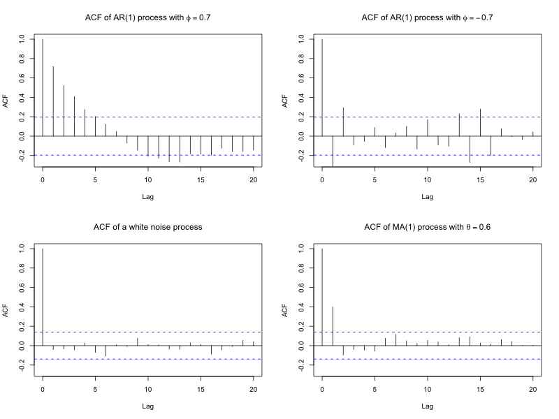
In an ACF plot, the x-axis indicate the different lags (e.g., lag 1, lag 2, lag 3, etc.), and the y-axis shows the strength of the autocorrelation. Thus, each bar in the ACF plot indicates the strength of the autocorrelation at a specific lag. The dotted lines in the ACF plot indicate \(95\%\) confidence bounds under the assumption that the data are generated by a [white noise] process (i.e., a process with no autocorrelation). If a bar falls outside these bounds, it suggests the autocorrelation at that lag is statistically significant with a significance level of \(0.05\).
1.2 What does the ACF tell you?
The ACF plot shows whether clear patterns or dependencies exist in your data over time. Specifically, it shows at which lags a variable is most related to its past values, how long past values continue to be related to current values, and whether the strength or direction of this relation changes across lags. Typically, autocorrelation decreases as the lag increases. However, it is also possible to see that there are certain seasonal or cyclic patterns in the data; for instance, when considering the ACF of daily diary data, you may observe a peak at lag 7, indicating that similar days in the week result in more similar scores than other days of the week.
In the time series literature, the ACF and PACF (to be discussed below) have been linked to the nature of an underlying process (Box & Jenkins, 1976). For example, it is known that a high autocorrelation at lag 1 that decreases exponentially toward zero suggests an AR(1) process with a positive \(\phi\) parameter. On the other hand, if the ACF shows a similar pattern of exponential decay as the lag increases but alternates in sign-negative at lag 1, positive at lag 2, and so on-this may indication of an AR(1) process with a negative \(\phi\) parameter. If the ACF shows a significant spike at lag 1 followed by non-significant autocorrelations at higher lags, this pattern is characteristic of a moving average process of order 1 (MA(1)). Similarly, if the ACF shows spikes at lag 1 and 2, followed by non-significant autocorrelations past these lags, the process may resemble a MA(2) process. However, empirical data rarely produces such idealized patterns, making the interpretation of the ACF plot as a diagnostic tool more complex and often ambiguous.
Amal has collected daily self-reports of stress levels from students over several weeks. Before diving into more advanced analyses, he wants to explore the structure of the data. To do so, he plots the ACF for each person separately. Amal notices that for most individuals the autocorrelation at lag 1 is high and positive, and that the autocorrelations decrease exponentially as the lag increases. Based on this pattern, Amal suspects that for most students, daily stress follows an autoregressive process with a positive \(\phi\) parameter.
In addition to visualizing temporal dependency patterns in the observed data, the ACF can also be used to inspect temporal dependencies in residuals (i,e., the portion of the data not explained by the model) after fitting a model such as an autoregression model. If the model has successfully captured the temporal structure that is present in the data, the residuals should resemble white noise: The ACF of the residuals should show no clear autocorrelation at any lag. If significant autocorrelations remain, this suggests the fitted model has not fully accounted for the temporal dependencies in the data, and a different or more complex model may be needed.
2 Partial autocorrelation
In addition to inspecting the autocorrelation, you can inspect the partial autocorrelation. The concept of the partial autocorrelation is similar to that of the partial correlation. While a partial correlation measures the unique correlation between two variables while controlling for other variables, the partial autocorrelation measures the unique correlation between the current values of a variable and its lagged values while controlling for all lags in between. In other words, the partial autocorrelation tells you how strong the current value is related to past values at a specific lag, while accounting for intermediate lags.
2.1 Partial autocorrelation function (PACF)
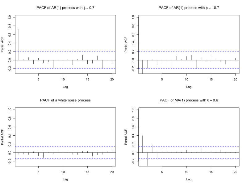
Like the autocorrelation can be computed at each lag and visualized, the partial autocorrelation can be computed at each lag using the partial autocorrelation function (PACF) and visualized. Figure 3 shows the PACF plots based on four different processes.
2.2 What does the PACF tell you?
The PACF plot shows the unique correlation between current values and a specific lag, accounting for all lags in between. Therefore, the PACF plot can be particularly useful to see which lagged values contribute new information beyond what has already been accounted for by intermediate lags. In the time series literature, the PACF plot is often used in combination with the ACF plot (Box & Jenkins, 1976).
At lag 1, the PACF is always identical to the ACF because there are no shorter, intermediate lags to accounted for. The distinction between the ACF and PACF becomes clearer at higher lags. For example, the ACF at lag 2 shows the correlation between current values and lagged 2 values. However, this autocorrelation could result from an indirect effect: It could be that the current values and lag 2 values are indirectly related through the effects of lag 1 echoing forward. The ACF agnostic to why there is an autocorrelation at lag 2, and thus does not inform you whether it is due to a direct or an indirect effect mediated by lag 1 (or a common cause, for that matter).
Inspecting the PACF helps clarify this. If the autocorrelation at lag 2 is entirely explained by lag 1, the PACF at lag 2 will show no partial autocorrelation, indicating no unique contribution from lag 2 once earlier lags are accounted for. In this way, the ACF and PACF provide complementary insights: The ACF shows overall autocorrelations at each lag, while the PACF isolates the unique contribution of each lag.
As with the ACF, specific models produce distinctive patterns in the PACF. These patterns could help identify both the type and order (i.e., the relevant lag) of the underlying process. For example, an AR model shows non-zero partial autocorrelations at the lags included in the model and zero partial autocorrelations beyond that point. That means an AR(1) process will show a spike at lag 1, followed by no partial autocorrelation at higher lags. An AR(2) process, will show spikes at lags 1 and 2, and no partial autocorrelations beyond lag 2. In this way, the number of significant spikes in the PACF can indicate the order of the AR model. In contrast, MA models show a different pattern: The PACF decreases gradually rather than cutting off at a specific lag. However, it remains important to keep in mind that real-world data rarely exhibit such idealized patterns, which makes interpreting the PACF in terms of a diagnostic tool more challenging in practice.
Leila has collected self-report measures of positive affect five times a day over two weeks. Before moving on to more detailed analysis, Leila wants to explore whether positive affect is directly influenced by specific earlier time points. She starts by looking at the ACF, which shows a noticeable positive autocorrelation at lag 2. This suggests that positive affect at a given time may be related to affect two measurements earlier. However, Leila knows this autocorrelation could be misleading. The positive autocorrelation at lag 2 might not reflect a direct relation between the current measurement and two time points earlier, but an indirect one, carried through lag 1.
To clarify this, Leila inspects the PACF. The PACF at lag 2 tells her whether positive affect at the current time point is still related to affect two measurements earlier, after accounting for all measurements in between. She finds that the PACF at lag 2 is near zero, which suggests there is no direct relation between those two time points: The apparent autocorrelation in the ACF at lag 2, was likely due to the lag 1 effects echoing forward.
3 Think more about
Estimating time series models used to be time-consuming and resource intensive before the era of computers (Box & Jenkins, 1976). This was especially the case if researchers wanted to compare autoregressive models with moving average models. Therefore, researchers relied heavily on the ACF and PACF to guide decisions on what type of model and which lags to include. In this context, the ACF and PACF mostly served as diagnostic tools.
With today’s fast-computing power, it has become much easier to fit multiple models to ILD and compare their performance. As a result, the use of the ACF and PACF as a diagnostic tool has diminished. Instead, the ACF and PACF are primarily used as an exploratory or descriptive tool, helping researchers visualize temporal patterns and dependencies in their data. Another important use of the ACF and PACF is to determine whether the residuals of a model behave as white noise, meaning that all temporal dependencies that were present in the data are accounted for by the model that was fitted.
Another way in which you may encounter autocorrelations is in the context of panel data. In that scenario, it is also a correlation between a variable and itself at another occasion, but instead of considering this within a single case across many occasions, it is computed across many cases, and at a single occasion with a single other occasion. You can read more about this difference in the article about the intra-indvidual versus inter-individual correlation.
4 Takeaway
The autocorrelation tells you if a variable is related to itself over time. The ACF and PACF are useful descriptive tools for summarizing temporal patterns in N=1 ILD. The ACF shows the overall dependencies between current and past values, helping you to detect whether, and for how long, previous states are related to the present. The PACF identifies the unique relations between specific lags while accounting for shorter-term lags. Together these measures provide a rich picture of how processes unfold over time and can guide your understanding of temporal dependencies before moving on to more complex modelling.
5 Further reading
We have collected various topics for you to read more about below.
Describing patterns in your intensive longitudinal data.
- Standard summary statistics
- [Cross-correlation function]
Modeling how current values depend on previous observations.
- Autoregressive model
- [ARIMA]
Acknowledgments
This work was supported by the European Research Council (ERC) Consolidator Grant awarded to E. L. Hamaker (ERC-2019-COG-865468).
References
Citation
@article{hoekstra2025,
  author = {Hoekstra, Ria H. A.},
  title = {Autocorrelation},
  journal = {MATILDA Preprints},
  number = {2025-05-23},
  date = {2025-05-23},
  url = {https://matilda.fss.uu.nl/articles/autocorrelation.html},
  langid = {en}
}