Types of variation

This article builds on Schuurman (2023)
This article is about different types of variation you may encounter when you study a given process. For example, the values of the constructs that are part of your process of interest may vary over time within a unit (e.g., a person), and may also vary across different units.
The different types of variation in constructs and processes are important to think about both when you want to measure them and when you want to analyze the ILD you obtained on them. For example, whether you measure a construct frequently enough will depend on how much its values change (vary) over time. And when you analyze your ILD, it is important to take into account whether characteristics of your process of interest, such as its mean value, differ from person to person or not (see homogeneity). More generally speaking, how constructs vary is a key characteristic of their distribution. Hence, it will be a key consideration for your sampling design and for determining what distributional assumptions are sensible when you analyze data on them.
Given its importance in the psychological literature, and on MATILDA, you will often encounter terminology related to these different types of variation and variance in processes and ILD collected on them. In this article, you can read more about how these terms can be defined and explained.
In this article, you will find: 1) the intra-individual variation and inter-individual variation; 2) within-person variance and between-person variance; 3) cross-sectional variance and grand variance; 4) how these four types of variance relate; and 5) how these four types of in terms of correlation relate.
1 Intra-individual differences versus inter-individual differences
In the literature people often refer to intra-individual differences or (interchangeably) variation, and inter-individual differences or variation. Intra-individual differences are differences that result from changes over time in the values of a construct.
Jan wants to know how to improve the reading ability of young children. To this end, he studies how the reading performance of a given child changes as the reading conditions of that child change. That is, he studies intra-individual differences in reading performance, and if these relate to intra-individual differences in various reading conditions.
For example, he finds that a child reading performance typically improves when they move from a noisy area to a quiet area. And, he finds that a child’s reading performance typically worsens when they read about a topic that the child finds ‘boring’, compared to when the child reads about a topic that interests them.
Inter-individual differences are differences in the values of a construct across different cases from a population, for example, across different persons.
Nur wants know how the home environment of children that generally perform well in reading, compare to those of children that generally perform poorly in reading. That is, Nur studies inter-individual differences in reading performance, and if these relate to inter-individual differences in children’s home environment.
For example, they find that children with high reading performance on average have more books in their homes compared to children with low reading performance. They also find that the parents of children with high reading performance on average enjoy and encourage reading for leisure more than the parents of children with low reading performance.
Importantly, intra-individual and inter-individual differences do not necessarily have to concern differences in the scores on a construct (such as in the previous examples), but may also concern differences in characteristics of processes. Notably, if a process is non-stationary, this would imply that there are intra-individual differences in the characteristics of that process. If a process is non-homogenous this would imply that there are inter-individual differences in the characteristics of that process.
In her studies, Achieng’ finds that the reading processes of children differ depending on whether they are reading for personal pleasure, or for a school assignment. When a child reads for pleasure, they take less breaks, read for longer periods of time, and have different eye movement patterns compared to when that child reads for a school assignment.
While analyzing the data, she finds that she needs a different model altogether when a child reads for pleasure, than when they read for a school assignment.
Minh studies how young children learn to read their first words. He finds that some children learn more words, and learn words more quickly than other children. He also finds that the effect of learning together with a small group of children on word acquisition differs from child to child: for some it slows their rate of acquisition, and for others it speeds up their rate of acquisition.
He takes these inter-individual differences into account in his model by allowing for different model parameters for different children. Their processes have different means, regression coefficients, and variances.
2 Within-person variance and between-person variance
In practice, variation is often quantified as a variance (for more info on what a variance is, see for example Wikipedia contributors, 2024). Below, different types of variation—and the variances based on this—are discussed that you can encounter in ILD studies. Throughout, the terms within-person and between-person are used, but this may also refer to other cases, for example dyads, organizations, or countries.
2.1 Within-person variance
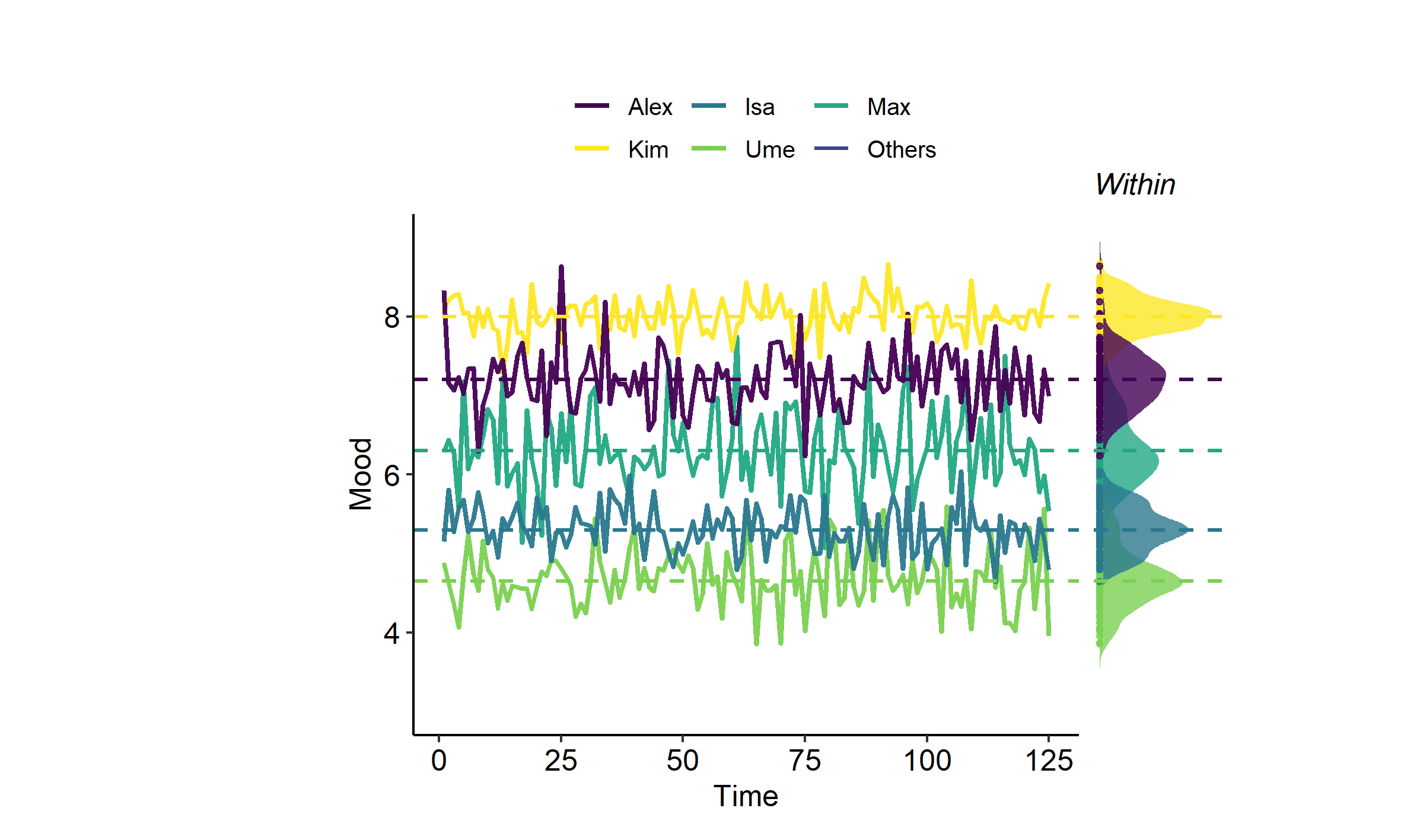
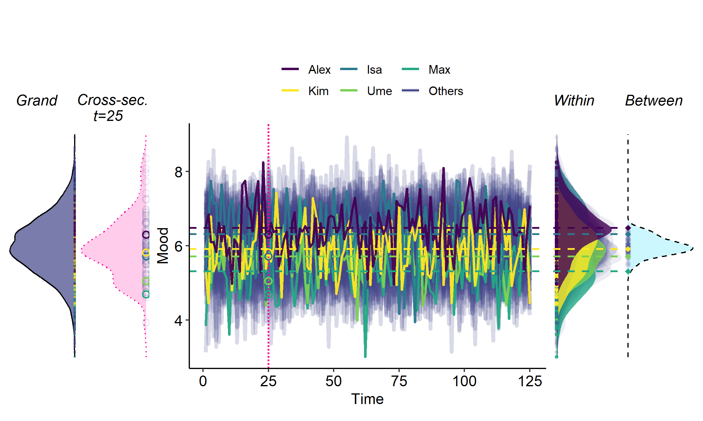
Within-person variation is variation over time in a person’s values for a given variable. When you quantify such variation with a variance, it is referred to as a within-person (or intra-individual) variance. The within-person variability and variance are illustrated for six different persons in Figure 1 below.
John rated his level of reading enjoyment on a scale from 1-7 each day for 5 days. The result is in the first two columns of the table below.
| Day | Enjoyment | \(( x - \bar{x} )\) | \((x - \bar{x})^2\) |
|---|---|---|---|
| 1 | 3 | -1.2 | 1.44 |
| 2 | 4 | -0.2 | 0.04 |
| 3 | 3 | -1.2 | 1.44 |
| 4 | 5 | 0.8 | 0.64 |
| 5 | 6 | 1.8 | 3.24 |
He applies the following equation for the variance to his five observations (note he uses the equation for the population rather than for a sample for his intents and purposes, see (ref:https://en.wikipedia.org/wiki/Variance)). In the equation, the concentration scores for specific day are indicated by \(x_{t}\).
\[\begin{equation} \text{Variance} = \frac{1}{n} \sum_{t=1}^{n} (x_t - \bar{x})^2 \end{equation}\]
First, John calculates his within-person mean (\(\bar{x}\)) concentration across the five days:
\[\begin{equation} \bar{x} = \frac{3 + 4 + 3 + 5 + 6}{5} = \frac{21}{5} = 4.2 \end{equation}\]
Next, he calculates the difference between the observed scores and their mean (column 3 of the above table), and then squares the result (column 4 of the above table). He then sums the results together, and divides by the number of repeated measures to obtain his within-person variance of concentration.
\[\begin{equation} \text{Within-person variance} = \frac{1}{n} \sum_{i=1}^{n} (x_t - \bar{x})^2 = \frac{1.44 + 0.04 + 1.44 + 0.64 + 3.24}{5} = \frac{6.8}{5} = 1.36 \end{equation}\]
2.2 Between-person variance
The term between-person variance has been used in the psychological literature in different ways, specifically to refer to:
- the variance of anything that varies across persons;
- the variance of the expected values of different persons.
Moreover, sometimes the term between-person variance may also be used to indicate a cross-sectional variance (see Section 3.1). It is therefore important to clearly state what variance you mean exactly when using this terminology.
2.2.1 Between-person variance as a variance of anything that varies across persons
Some researchers define between-person variance as the variance of anything that varies across persons. That is, when you define between-person variance in this way, it is simply the variance of something that varies from person to person. That could be different people’s scores at a given point in time, but also the variance of the parameters of different people.
James presented his new children’s book to five children: Elena, Susan, Riley, Han and Gahungu. When they finished the book, each child rated their level of reading enjoyment on a scale from 1-10. The result is in the first two columns of the table below.
| Child | Enjoyment | \(( x - \bar{x} )\) | \((x - \bar{x})^2\) |
|---|---|---|---|
| Elena | 7 | -0.4 | 0.16 |
| Susan | 5 | -2.4 | 5.76 |
| Riley | 9 | 1.6 | 2.56 |
| Han | 6 | -1.4 | 1.96 |
| Gahungu | 8 | 0.6 | 0.36 |
James applies the following equation for the variance to the children’s scores. In the equation, the enjoyment scores for specific child are indicated by \(x_{i}\).
\[\begin{equation} \text{Variance} = \frac{1}{n} \sum_{i=1}^{n} (x_i - \bar{x})^2 \end{equation}\]
First, James calculates the average enjoyment score (\(\bar{x}\)) across the five children:
\[\begin{equation} \bar{x} = \frac{7 + 5 + 9 + 6 + 8}{5} = \frac{35}{5} = 7 \end{equation}\]
Next, he calculates the difference between the observed scores and their mean (column 3 of the above table), and then squares the result (column 4 of the above table). He then sums the results together, and divides by the number of children to obtain the between-person variance of reading enjoyment scores.
\[\begin{equation} \text{between-person variance} = \frac{1}{n} \sum_{i=1}^{n} (x_i - \bar{x})^2 = \frac{0.16 + 5.76 + 2.56 + 1.96 + 0.36}{5} = \frac{10.8}{5} = 2.16 \end{equation}\]
Note: This between-person variance can also be considered a cross-sectional variance, given that we calculate the variance of observed scores of different persons at one point in time.
Petra has collected intensive longitudinal data, consisting of 70 repeated measures of reading enjoyment of five elementary school children. She wants to know how much between-person variability there is in the autoregression coefficients of their reading enjoyment.
She has analyzed each child’s data with an AR(1) model and has obtained the autoregression coefficients (\(\phi\)) for each child, which are presented in the second column in the table below. She proceeds by calculating the between-person variance over the different autoregression coefficients.
She applies the following equation for the variance to the children’s autoregression coefficients (which are indicated with \(\phi_{i}\)).
\[\begin{equation} \text{Variance} = \frac{1}{n} \sum_{i=1}^{n} (\phi_i - \bar{\phi})^2 \end{equation}\]
| Child | \(( \phi - \bar{\phi} )\) | \((\phi - \bar{\phi})^2\) | |
|---|---|---|---|
| Amina | 0.5 | -0.04 | 0.0016 |
| Leo | 0.7 | 0.16 | 0.0256 |
| Priya | 0.3 | -0.24 | 0.0576 |
| Jonas | 0.8 | 0.26 | 0.0676 |
| Fatima | 0.4 | -0.14 | 0.0196 |
First, Petra calculates the average autoregression coefficient (\(\bar{\phi}\)) across the five children:
\[\begin{equation} \bar{\phi} = \frac{0.5 + 0.7 + 0.3 + 0.8 + 0.4}{5} = \frac{2.7}{5} = 0.54 \end{equation}\]
Next, she calculates the difference between the autoregression coefficients and this mean (column 3 of the above table), and then squares the result (column 4 of the above table). She then sums the results together, and divides by the number of children to obtain the between-person variance of reading enjoyment autoregression coefficients.
\[\begin{equation} \begin{split} \text{between-person variance} &= \frac{1}{n} \sum_{i=1}^{n} (\phi_i - \bar{\phi})^2\\ & = \frac{0.0016 + 0.0256 + 0.0576 + 0.0676 + 0.0196}{5} = \frac{0.172}{5} = 0.0344\end{split} \end{equation}\]
This a very general and liberal definition of a between-person variance. It is important to note that in the psychological literature, some people mean something more specific with this terminology instead (see Section 2.2).
2.2.2 Between-person variance as the variance of different persons’ expected values
In this definition of between-person variance, it is the variance of different persons’ expected values for a given construct. Equivalently, you may see this denoted as the variance of different persons’ means for a given construct, where the means are calculated over each person’s repeated measures.
This is a definition of the between-person variance that you will often encounter in the ILD and multilevel modeling literature, especially in the context of [separating within- and between-person level variance], and the ecological fallacy. In those contexts you may also see this variance referred to as ‘trait variance’ or the variance of ‘stable between-person differences’: This is based on the idea that the means reflect a time-stable, trait-like characteristic of each person.
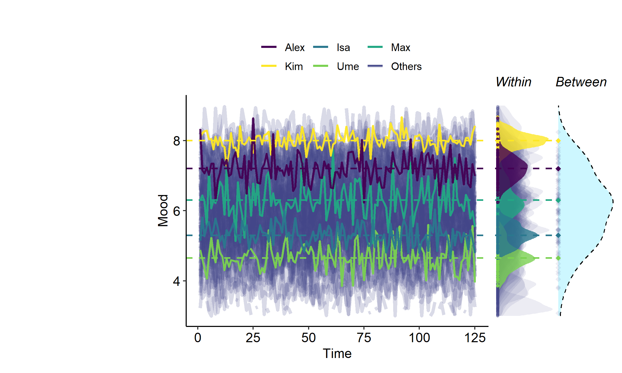
Consider that each participant in an ILD data set has a mean score over their repeated measures for a particular variable. If you calculate the variance across these means of the different persons, you have calculated their between person variance, according to this definition. This is illustrated in Figure 2 below.
Petra has collected intensive longitudinal data, consisting of 70 repeated measures of reading enjoyment of five elementary school children. She wants to know how much between-person variability there is in their means (their expected values) of their reading enjoyment.
First, she has calculated the mean reading enjoyment for each child by taking the mean over their respective 70 repeated measures of enjoyment. She proceeds by calculating the between-person variance over the different children’s means (\(\mu_i\)).
She applies the following equation for the variance to the children’s means (which are indicated with \(\mu_{i}\)).
\[\begin{equation} \text{Variance} = \frac{1}{n} \sum_{i=1}^{n} (\phi_i - \bar{\phi})^2 \end{equation}\]
| Child | \(\mu\) | \(( \mu - \bar{\mu} )\) | \((\mu - \bar{\mu})^2\) |
|---|---|---|---|
| Amina | 6 | 0.2 | 0.04 |
| Leo | 8 | 2.2 | 4.84 |
| Priya | 3 | -2.8 | 7.84 |
| Jonas | 7 | 1.2 | 1.44 |
| Fatima | 5 | -0.8 | 0.64 |
First, Petra calculates the average mean (\(\bar{\mu}\)) across the five children:
\[\begin{equation} \bar{\mu} = \frac{6 + 8 + 3 + 7 + 5}{5} = \frac{29}{5} = 5.8 \end{equation}\]
Next, she calculates the difference between the children’s means and this average mean (column 3 of the above table), and then squares the result (column 4 of the above table). She then sums the results together, and divides by the number of children to obtain the between-person variance.
\[\begin{equation} \begin{split} \text{between-person variance} &= \frac{1}{n} \sum_{i=1}^{n} (\mu_i - \bar{\mu})^2 &= \frac{0.04 + 4.84 + 7.84 + 1.44 + 0.64}{5} = \frac{14.8}{5} = 2.96 \end{split} \end{equation}\]
This a narrow and specific definition of the term between-person variance. It is important to realize that in the general psychological literature, people may mean something else with this terminology instead (see Section 2.2).
3 Cross-sectional variance and grand variance
For a given set of ILD you can consider not only between-person variance(s) and within-person variance(s), but also the cross-sectional variance, and the grand variance. The latter two are describe in more detail below.
3.1 Cross-sectional variance
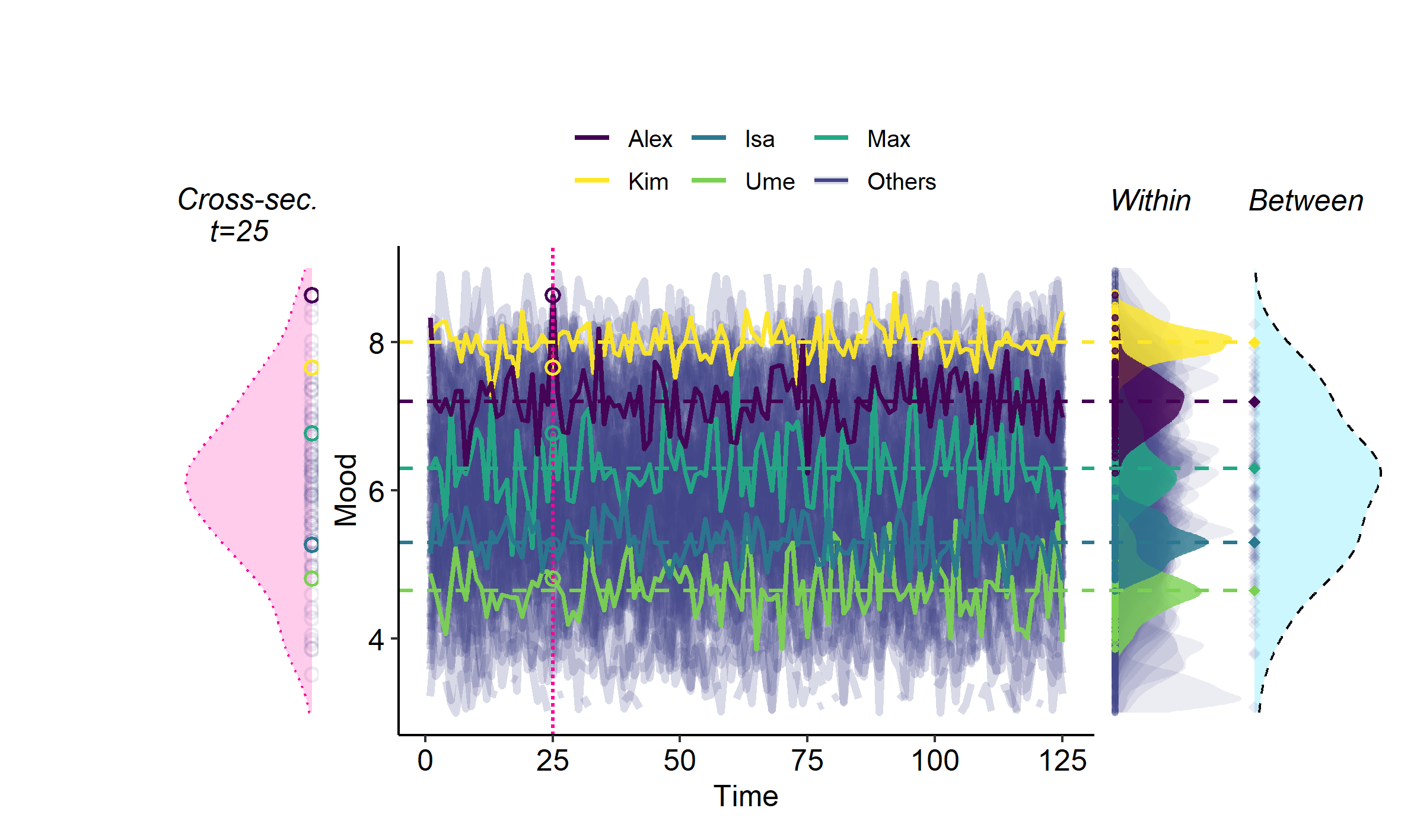
The cross-sectional variance is the variance taken over the values of a variable at one particular point in time, across persons (or other cases): It is the type of variance you obtain if you do a cross-sectional study. The cross-sectional variance is illustrated in Figure 3 below for ILD.
Note that for ILD with multiple persons, you can actually calculate a cross-sectional variance at each measurement occasion.
Ari has collected three repeated measures of reading ability for three different children. You see the result below.
| Child | Time | Reading ability (\(x\)) |
|---|---|---|
| 1 | 1 | 6 |
| 1 | 2 | 8 |
| 1 | 3 | 7 |
| 2 | 1 | 4 |
| 2 | 2 | 5 |
| 2 | 3 | 6 |
| 3 | 1 | 9 |
| 3 | 2 | 7 |
| 3 | 3 | 8 |
Ari can calculate three cross-sectional variances based on this example data set: The cross-sectional variance for time point 1, 2 and 3. We illustrate how this is done for the cross-sectional variance of time point 1.
First, Ari extract the scores for the different persons at time point 1 and calculates the mean of these scores:
\[\begin{equation} \bar{\x} = \frac{6 + 4 + 9}{3} = \frac{19}{3} \approx 6.33 \end{equation}\]
Then, Ari calculates the cross-sectional variance:
\[\begin{equation} \begin{split} \text{cross-sectional variance} &= \frac{1}{n} \sum_{i=1}^{n} (x_i - \bar{x})^2 &= \frac{0.1089 + 5.4289 + 7.1289}{3} = \frac{12.6667}{3} \approx 4.22 \end{split} \end{equation}\]
Ari can also do this for time point 2 and 3. The results are presented in the table below.
| Time point | Cross-sectional mean | Cross-sectional variance |
|---|---|---|
| 1 | 6.33 | 4.22 |
| 2 | 6.67 | 1.55 |
| 3 | 7.00 | 0.67 |
Note: Of course this basic idea generalizes to intensive longitudinal data, where we have many more repeated measures and more persons. However, that would result in a huge table for this example!
3.2 Grand variance
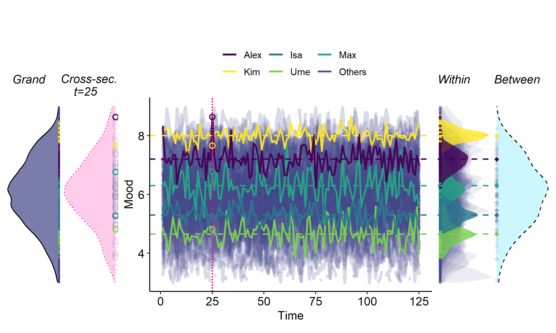
The grand variance is the variance taken over all occasions for all persons (or other cases) for a variable. Hence, it is the variance taken over all observations in the dataset for a given variable. This is illustrated in Figure 4 below.
Ari has collected three repeated measures of reading ability for three different children. You see the result below.
| Child | Time | Reading ability (\(x\)) |
|---|---|---|
| 1 | 1 | 6 |
| 1 | 2 | 8 |
| 1 | 3 | 7 |
| 2 | 1 | 4 |
| 2 | 2 | 5 |
| 2 | 3 | 6 |
| 3 | 1 | 9 |
| 3 | 2 | 7 |
| 3 | 3 | 8 |
Ari calculates the grand variance of reading ability by simply calculating the variance over all scores in the data set.
First, he calculates the grand mean (\(\bar{x}\)) over all of the observed scores (\(x_i\)): \[\begin{equation} \begin{split} \bar{\x} &= \frac{6 + 8 + 7 + 4 + 5 + 6 + 9 + 7 + 8}{9} &=\frac{60}{9} = 6.\overline{6} \end{split} \end{equation}\]
Then he calculates the grand variance as follows: \[\begin{equation} \text{grand variance} = \frac{1}{9} \sum_{i=1}^{9} (x_i - \bar{x})^2 = \frac{20}{9} \approx 2.22 \end{equation}\]
Note: Of course this basic idea generalizes to intensive longitudinal data, where we have many more repeated measures and more persons. However, that would result in a huge table for this example!
4 How the within-person, between-person, grand and cross-sectional variance relate
The within-person variance(s), between-person variance (as defined in Section 2.2.2), cross-sectional and grand variance are all related to each other.
In particular, because the grand variance is taken both over the occasions of each person, and over the scores across different persons, it will consist of both within-person variability and between-person variability. This also applies to the cross-sectional variance, because the cross-sectional variance is a special case of the grand variance.
To get a better understanding of this, consider the scenario where individuals are characterized by a stationary process of the same functional form (the same model), except that each person may have their own unique parameter values.1 As an example, suppose that each person in your population of interest has an autoregressive process for variable mood, but they have person-specific means and autoregressive coefficients.
In such a scenario, you can simplify the process for variable \(y\) (for example mood), which varies over persons \(i\) and occasions \(t\) as follows:
\[\begin{equation} \label{eq:sum} y_{it} = b_{i} + w_{it}. \end{equation}\]
Here, \(b_{i}\) is the person-specific mean or expected value of variable \(y_{it}\) for person \(i\), and \(w_{it}\) is the deviation from that mean for person \(i\) at occasion \(t\).
The term \(b_i\) represents the between-persons part of the variable \(y\): These person-specific means reflect differences between persons that are stable over time. The term \(w_{it}\) represents the within-person part of variable \(y\): It captures fluctuations around the person’s mean over time, and it could be governed by any (stationary) dynamic process, such as an autoregressive process.
It has been shown that, for such a stationary process, the grand variance and cross-sectional variance of \(y\) are equal,2 and that they are the sum of (see Schuurman et al., 2016; Schuurman, 2023):
the between-person variance: the variance taken over the means of the different persons;
the average within-person variance; this is based on first obtaining the within-person variance for each person, and then taking the average over those variances.
You can see this from Figure 4, where the grand and cross-sectional distributions have the same width, which will generally be true for stationary processes as described in this section.
You may also notice from Figure 4 that the width of the grand and cross-sectional distributions look similar—but this is a feature of that particular example, that is not generally the case (!). The grand or cross-sectional will simply resemble the between-variance when the average within-person variance is relatively small, and it will resemble the average within-person variance when the between-variance is relatively small. This is illustrated in another example visualized in Figure 5 below.
You can also try out yourself how cross-sectional or grand distributions change when you change the amount of within-person or between-person variance.
To this end, go to the middle tab “univariate normal densities” in this Shiny app.
5 How the within-person, between-person, grand and cross-sectional correlation relate
The above can also be extended to multiple variables and their covariances, and to the correlations that follow from this (see Hamaker, 2024; Schuurman et al., 2016; Schuurman, 2023 for details).
It can be shown that the grand or cross-sectional correlation between two variables is a complex combination of:
the between-person correlation: the correlation between the means for each variable of different people. This correlation captures whether people who have a high mean on one variable also tend to have a high mean on the other variable, and vice versa.
the average within-person correlation: the average of each person’s within-person correlation. The within-person correlation can differ across persons. These correlations capture whether when a particular person has a high score on one variable, they simultaneously tend to have a high score on the other variable, and vice versa.
Whether the cross-sectional or grand correlation resembles the between-person correlation, the average within-person correlation, or neither, depends on how much between- and within-person variance there is for each of the variables.
Typically, the value of the cross-sectional or grand correlation will lie in between that of the within-person and between-person correlation, but this is not necessarily the case (Hamaker, 2024). If there is relatively a lot of between-person variance for both variables the correlation will resemble the between-person correlation the most. When there is relatively a lot of within-person variance for both variables the correlation will resemble the average within-person correlation the most.
If there is a lot of between-person variance for one variable, and a lot of within-person variance for another variable, the cross-sectional correlation may resemble neither correlation very well. Moreover, when the between-person correlation and the within-person correlation are very similar, it is very likely that the cross-sectional correlation will actually not fall between them, but that it ends up being closer to zero than both of them (Hamaker, 2024).
You can also try out yourself how cross-sectional or grand correlations change when you change the amount of within-person or between-person variance.
To this end, go to this Shiny app.
You can also consider correlations between variables measured at different occasions, or between the same variable at different occasions. This is further discussed in the article on inter-individual and intra-individual correlations.
6 Think more about
For your study, it is of essential important to think about how your process varies and what variation you are interested in based on your research question and goals. What kind of variation and how much variation you end up with in your data, will to a large extent depend on how you designed your measurement instrument. Next to this, you can also use statistical techniques to separate out and target different types of variance, such as multilevel modeling (see Schuurman, 2023). This is important to avoid the [within/between problem] and committing the [ecological fallacy].
Different types of studies traditionally often focus on different types of data, that emphasize different types variation. For example, cross-sectional studies use inter-individual difference data, and tend to focus on between-person variance (as in Section 2.2.2). ILD studies typically focus on intra-individual differences and within-person variance(s), but may also study inter-individual differences and between-person variance (either definition discussed in Section 2.2). For example, in ILD studies it is common to investigate how a process and all its parameters differs from person to person with a multilevel model.
7 Takeaway
When you study processes with ILD there are different types of variation to consider: differences among persons (or other cases), or differences over time. Such differences can be quantified with different types of variances.
Notably, different authors in the literature may use the same terminology to mean the variances of different things, particularly for the ‘between-person variance’. It is important to get clear which one is meant, because they contain different information.
Similarly, for your ILD study, it is of essential importance to think about how your process varies and what variation you are interested in based on your research question and goals.
Importantly, when you calculate the variance for data based on multiple people (even if you only consider one occasion), you should expect it to potentially consist of both between-person and within-person variance. If you are interested in either of these variances, or both, rather than their combination, you should think about the [within/between problem] and the [ecological fallacy].
8 Further reading
We have collected various topics for you to read more about below.
- Ecological fallacy
- [The within/between problem]
References
Footnotes
Note that these variances are also related in the context of non-stationary processes, and also in that scenario (even more so) the ecological fallacy and within/between problem are important to consider. However, that scenario is more complex (see Schuurman, 2023).↩︎
Note: in a particular sample they may differ a bit, but this is due to sampling error.↩︎
Citation
@article{schuurman2025,
  author = {Schuurman, Noémi K.},
  title = {Types of Variation},
  journal = {MATILDA Preprints},
  number = {2025-05-23},
  date = {2025-05-23},
  url = {https://matilda.fss.uu.nl/articles/types-of-variation.html},
  langid = {en}
}