
Regime-switching autoregressive model with intercept versus mean
This article is about regime-switching autoregressive (AR) models, and how the behavior of such models depends on which formulation you use for the AR processes. An AR model can be either expressed with lagged versions of the observed variable as its predictors, or with lagged versions of the mean-centered observed variable as its predictors. The former includes an intercept that represent the expected value for the outcome when all the observed lagged predictors are zero, while the latter includes the long-run mean of the process that represents the expected value for the outcome when all mean-centered lagged predictors are zero. For linear models, these two formulations are mathematically identical, where one is simply a reparameterization of the other; you can read more about this in the article about two formulations of an AR model.
However, the equivalence between these two breaks down when there are regime-switches. In particular, a regime-switching AR model with lagged versions of the observed variable as its predictors results in a somewhat gradual transitions towards the new equilibrium in the observed series, even though the underlying regime switch is sudden. In contrast, having lagged versions of mean-centered observations as the predictors results in an almost instantaneous shift between regimes in the observed series, reflecting the underlying sudden shift. Understanding this is particularly relevant if you want to use a regime-switching AR model, such as a Markov-switching autoregressive (MS-AR) model, or a threshold autoregressive (TAR) model, because it has implications for the temporal patterns that these different models can generate—and thus account for when used to analyze empirical data.
To help you gain more insight into these matters, below you can read about: 1) a brief recap of the different representations of an AR model; 2) an extension of the AR model that includes regime-switching, with an example showing that the model based on expressions with intercepts allows for more smooth regime-switches than the model based on expressions with means; 3) a mathematical derivation and graphical explanation of the behavior of a regime-switching AR model with an intercept for each regime; and 4) how a minor model tweak for the model with a mean per regime results in a version that is identical to the regime-switching model with an intercept per regime.
1 Two representations of an AR model and their connection
There are two ways in which an AR model can be represented; this is discussed in more detail in the article about the two formulations of an AR model. Here, a minor recap is presented. For simplicity, the focus is limited to first-order autoregressive (AR(1)) models; therefore, the subscript 1 for the autoregressive parameter will be omitted throughout.
A common way to represent an AR(1) model is
\[y_t = c + \phi y_{t-1} + \epsilon_t,\]
where the intercept \(c\) represents the value you should expect for \(y_t\) if \(y_{t-1}=0\). While this may be of interest at times, quite often the intercepts does not have much appeal from a substantive perspective.
An alternative way to represent an AR(1) model is by regressing the outcome on the lagged mean-centered version of itself. When \(\mu\) is the mean of the AR(1) process, this can be written as
\[ y_t = \mu + \phi \bigl( y_{t-1} - \mu \bigr) + \epsilon_t.\]
This clearly shows that when \(y_{t-1} = \mu\), then the value you should expect for \(y_t\) is \(\mu\). In words, this implies that when the previous observations was equal to the long-run mean, the expected value for the current observation is also the long-run mean.
To see how \(c\) and \(\mu\) are connected, you can rewrite the latter expression as
\[ y_t = \mu -\phi \mu + \phi y_{t-1} + \epsilon_t.\]
which shows the \(c=(1-\phi)\mu\), and thus \(\mu=c/(1-\phi)\).
The two versions of an AR model—whether using \(y_{t-1}\) and involving the intercept \(c\), or using \(y_{t-1}-\mu\) and involving the mean \(\mu\)—are mathematically equivalent; you can read more about this in the article about the two formulations of an AR model. This equivalence also holds when there is displacement in an AR model, which means that the process is moved far away from its long-run mean \(\mu\). In that case, both formulations account for the exact same gradual progression towards the long-run equilibrium of the AR model.
Given this model equivalence between the two formulations for linear AR models, it may be puzzling that this equivalence does not generalize to regime-switching AR models. In the following sections you can see the different behaviors of the two formulations of a regime-switching AR model in detail, as well as an explanation of where this difference is actually coming from.
2 Regime-switching with intercepts or means
The model equivalence presented above for the linear AR model does not generalize to the non-linear case, such as a regime-switching AR model. In this section, first the two formulations of a regime-switching AR(1) model are presented. Subsequently, a numerical example is presented that shows how the two formulations lead to different behavior after a switch.
2.1 Two formulations of a regime-switching AR(1) process
As with the linear AR(1) model, the regime-switching AR(1) process can also be formulated in two ways. To show that parameters may differ across regimes, the subscript \((S_t)\) is included, where \(S_t=1,2,\dots,K\) to indicate the regime the process is in at occasion \(t\).
Building on the first expression for an AR(1) model, which includes a lagged version of the observed variable as the predictor, the regime-switching AR(1) model can be written as
\[y_t = c_{(S_t)} + \phi_{(S_t)} y_{t-1} + \epsilon_t,\]
where both the intercept and the autoregressive parameter depend on the regime the process is in. When the process remains in the same regime for a very long time, the process will eventually fluctuate around its long-run regime-specific equilibrium, which is
\[\mu_{(S_t)} = \frac{c_{(S_t)}}{1-\phi_{(S_t)}}.\]
Alternatively, when considering the second expression for an AR(1) model and extending this to a regime-switching version, this gives you
\[y_t = \mu_{(S_t)} + \phi_{(S_t)}(y_{t-1} - \mu_{(S_{t-1})}) + \epsilon_t .\]
What is important to note when considering this expression, is that the two long-run means on the right-hand side are not necessarily the same, as indicated by their different subscripts. When \(y_t\) and \(y_{t-1}\) come from the same regime, meaning \(S_t = S_{t-1}\), than the two long-run means are the same. However, when a switch occurred between \(t-1\) and \(t\), then \(S_t \neq S_{t-1}\) and thus \(\mu_{(S_t)} \neq \mu_{(S_{t-1})}\). This has major consequences (and you can also see in one of the sections below what happens if you use the same mean instead).
2.2 Numerical example of a regime-switching AR(1) process
In Figure 1 you can see two time series that were generated with the same sequence of innovations. The red series is based on the expression with an intercept, using \(c_{(1)} = 5\) and \(\phi_{(1)}=0.5\) for the first regime so that its long-run mean would be \(\mu_{(1)}=5/0.5=10\), combined with \(c_{(2)} = 10\) and \(\phi_{(2)}=0.6\) for the second regime so that its long-run mean would be \(\mu_{(2)}=10/0.4=25\). The blue series is based on the expression with means and has the same autoregressive parameters as the red series, and the regime means that are the same as the long-run means from as the red series, that is, \(\mu_{(1)}=10\) and \(\mu_{(2)}=25\).
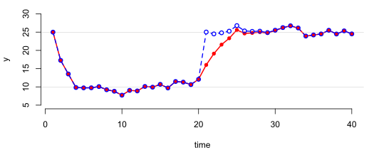
Both series start in the first regime, and both switch to the second regime after \(t=20\). The initial value of both series is \(y_1=25\), which can be considered a substantial displacement from the long-run mean of the first regime. The sequences in Figure 1 show that the two series behave identical until the regime switch. This is in agreement with results presented in the article about how displacement of an AR model affects the trajectory that is generated with each of the two formulations of an AR process.
However, the series in Figure 1 diverge right after the switch: Whereas the series represented in blue (based on an expression with the long-run means per regime) is characterized by a complete and instant switch to the new regime, the series in red (based on an expression with intercepts per regime) is characterized by a transition period during which the process gradually climbs towards the long-run equilibrium that characterizes the second regime. Interestingly, after about ten occasions, the two series are virtually identical again.
This implies that a process that is characterized by a sudden switch from one state to another—each of them being characterized by its own equilibrium or attractor, and by its own dynamics around this—does not have to show abrupt switching in the observed series: The regime-switching models with an intercept per regime allow for somewhat smoother transitions from one regime to another, depending on the degree of autoregression in a regime. However, sudden switching in the observed series is also a possibility; this results from a regime switching model based on having means rather than intercepts, and thus centered rather than uncentered lagged predictors.
Leatitia is interested in the way a person’s affective state changes when they enter a depressive episode. She wonders whether this can be considered a rather sudden switch from one day to the next, or that this is better understood as a gradual worsening of symptoms until a state of full-blown depression is reached.
Leatitia is wondering what model to use for the change from a symptom-free state to a depressed state. She thinks a regime-switching AR model would be particularly useful for this, but she is not sure whether to use a version that allows for a more gradual transition or one that implies a sudden change in symptom level. Actually, she would like to compare these two options to determine which one fits the temporal pattern in the data better.
To do so, Leatitia looks for a regime-switching state-space model, as described by Kim & Nelson (1999): Using this set-up, she can specify a model that allows for gradual change by including an intercept in the transition equation, whereas she can specify a model that implies a sudden change by including a long-run mean in the measurement equation and combining this with autoregressive residuals in the transition equation.
3 Trajectory after the regime switch when there is an intercept
To see why the regime-switching AR(1) model with intercepts and the uncentered lagged predictors results in a trajectory towards the new long-run equilibrium rather than a sudden switch, it helps to determine how the expected value of \(y\) evolves in the occasions following a regime switch. In what follows, the expected value for \(y_t\) is derived, starting with the scenario in which no switch has taken place yet, followed by the scenario when a switch has just occurred prior to the current occasion, then the scenario when the switch occurred the occasion before that, and so on.
This helps to see how the expectation of \(y\) changes as the regime switch took place further and further into the past. Alternatively, you could also consider the pattern of expectations when fixing the timing of the switch and find the expressions for \(y_{t+1}\), \(y_{t+2}\), and so on; while this would result in the same pattern of expectations, it would appear more messy as you would you would have to consider the effects of past innovations on future outcomes, resulting in expressions like \(\epsilon_{t+2-1}\) and \(\epsilon_{t+3-3}\) et cetera.
The mathematical derivations presented below are still somewhat involved, but they are also visualized using path diagrams. You can also decide to jump to the end of this section, where the general result is summarized.
3.1 When no switch has taken place yet
When no switch between regimes has taken place yet, and the process is in the first regime, the expected value for \(y_t\) can be found through the following approach. As point of departure, you take the expression of the AR(1) model in the first regime, that is
\[y_t = c_{(1)} + \phi_{(1)} y_{t-1} + \epsilon_t.\]
The lagged variable can be expressed similarly as \(y_(t-1)= c_{(1)} + \phi_{(1)} y_{t-2} + \epsilon_{t_1}\), which includes itself a lagged predictor that can be expresses as \(y_(t-2)= c_{(1)} + \phi_{(1)} y_{t-3} + \epsilon_{t_2}\). Repeatedly entering these into the expression for \(y_t\), you obtain the infinite expression
\[y_t = c_{(1)} + \epsilon_t + \phi_{(1)} ( c_{(1)} + \epsilon_{t-1} ) + \phi_{(1)}^2 ( c_{(1)} + \epsilon_{t-2} )+ \phi_{(1)}^3 ( c_{(1)} + \epsilon_{t-3}) + \dots\]
Collecting all the terms with c together, you get
\[y_t = (1 + \phi_{(1)} + \phi_{(1)}^2 + \phi_{(1)}^3 + \dots ) c_{(1)} + \epsilon_t + \phi_{(1)} \epsilon_{t-1} + \phi_{(1)}^2 \epsilon_{t-2} + \phi_{(1)}^3 \epsilon_{t-3} + \dots\]
When taking the expectation of this expression, all the terms containing innovations become zero, whereas the first term only contains constants, so you get
\[E[y_t] = (1 + \phi_{(1)} + \phi_{(1)}^2 + \phi_{(1)}^3 + \dots ) c_{(1)}. \]
When \(-1<\phi_{(1)}<1\), then the infinite sum of increasing powers of \(\phi_{(1)}\) is known in the mathematical literature as a geometric series, which converges to
\[ E[y_t] = \frac{c_{(1)}}{1-\phi_{(1)}}.\]
This forms the expression of the long-run equilibrium value or mean of the first regime.
3.2 When the switch took place between \(t-1\) and \(t\)
Suppose the change took place just before the current occasion \(t\). This gives
\(y_t = c_{(2)} + \epsilon_t + \phi_{(2)}(c_{(1)} + \epsilon_{t-1}) +\phi_{(2)}\phi_{(1)}(c_{(1)} + \epsilon_{t-2}) + \phi_{(2)}\phi_{(1)}^2(c_{(1)} + \epsilon_{t-3}) + \phi_{(2)}\phi_{(1)}^3(c_{(1)} + \epsilon_{t-4}) + \dots\)
\(\;\;\;\; = c_{(2)} + \epsilon_t + \phi_{(2)} \Big[(c_{(1)} + \epsilon_{t-1}) +\phi_{(1)}(c_{(1)} + \epsilon_{t-2}) + \phi_{(1)}^2(c_{(1)} + \epsilon_{t-3}) + \phi_{(1)}^3(c_{(1)} + \epsilon_{t-4}) + \dots \Big]\)
\(\;\;\;\; = c_{(2)} + \phi_{(2)} \Big[c_{(1)} +\phi_{(1)}c_{(1)} + \phi_{(1)}^2c_{(1)} + \phi_{(1)}^3c_{(1)} + \dots \Big] + \epsilon_t + \phi_{(2)} \Big[ \epsilon_{t-1} +\phi_{(1)} \epsilon_{t-2} + \phi_{(1)}^2 \epsilon_{t-3} + \phi_{(1)}^3 \epsilon_{t-4} + \dots \Big]\)
This expression can be visualized as in Figure 2. It shows that \(c_{(2)}\) only has a direct effect on \(y_t\), whereas \(c_{(1)}\) only has indirect effects, all of which go through the arrow \(\phi_{(2)}\) that connects \(y_{t-1}\) with \(y_t\). These indirect effects go through past versions of \(y\), infinitely far back in time; yet, the further back in time, the smaller the effect as it is based on a longer chain of \(\phi_{(1)}\)’s (which by definition lies between -1 and 1).
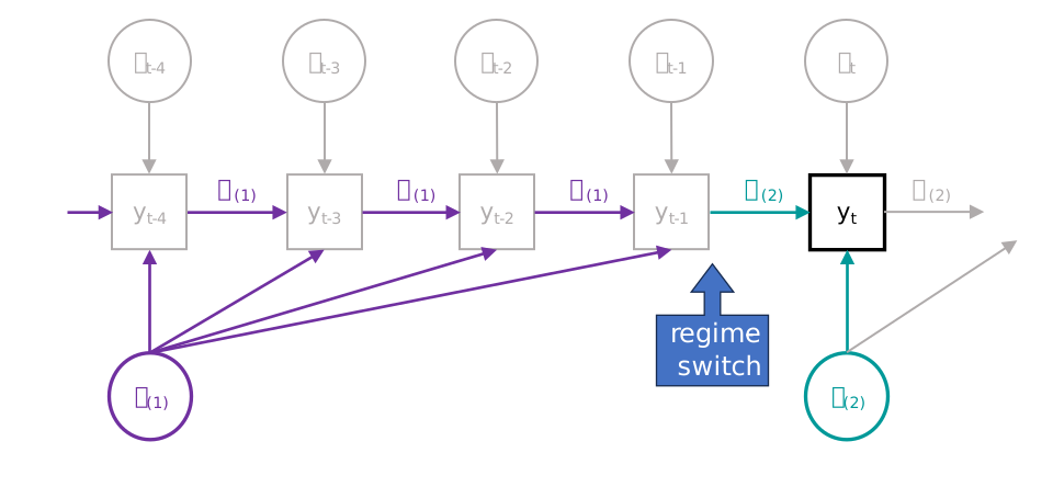
If you take the expectation of the expression given above for \(y_t\), the second half (which contains the innovations) becomes zero; this is why these are grayed out in Figure 2. Moreover, the second term on the right-hand side contains a geometric series again, so you get
\[E[y_t] = c_{(2)} + \phi_{(2)}\frac{c_{(1)}}{1-\phi_{(1)}}.\]
This represents the score you can expect for \(y_t\) when the switch from first to the second regime has just taken place. This expected value should thus not be confused with the long-run mean of the second regime; instead it represents a transitional expected value that still reflects the influence of the first regime. As time progresses, this influence fades, as you can see in the following scenarios.
3.3 When the switch took place between \(t-2\) and \(t-1\)
If the switch took place one occasion earlier—between \(t-2\) and \(t-1\)—you get
\(y_t = c_{(2)} + \epsilon_t + \phi_{(2)}(c_{(2)} + \epsilon_{t-1}) +\phi_{(2)}^2(c_{(1)} + \epsilon_{t-2}) + \phi_{(2)}^2\phi_{(1)}(c_{(1)} + \epsilon_{t-3}) + \phi_{(2)}^2\phi_{(1)}^2(c_{(1)} + \epsilon_{t-4}) + \dots\)
\(\;\;\;\; = c_{(2)} + \epsilon_t + \phi_{(2)}(c_{(2)} + \epsilon_{t-1}) + \phi_{(2)}^2 \Big[(c_{(1)} + \epsilon_{t-2}) + \phi_{(1)}(c_{(1)} + \epsilon_{t-3}) + \phi_{(1)}^2(c_{(1)} + \epsilon_{t-4}) + \dots \Big]\)
\(\;\;\;\; = c_{(2)} + \epsilon_t + \phi_{(2)}(c_{(2)} + \epsilon_{t-1}) + \phi_{(2)}^2 \Big[c_{(1)} +\phi_{(1)}c_{(1)} + \phi_{(1)}^2c_{(1)} + \dots \Big] + \phi_{(2)}^2 \Big[ \epsilon_{t-2} + \phi_{(1)} \epsilon_{t-3} + \phi_{(1)}^2 \epsilon_{t-4} + \dots \Big]\)
\(\;\;\;\; = c_{(2)} + \phi_{(2)}c_{(2)} + \phi_{(2)}^2 \frac{c_{(1)}}{1-\phi_{(1)}} + \epsilon_t + \phi_{(2)} \epsilon_{t-1} + \phi_{(2)}^2 \Big[ \epsilon_{t-2} + \phi_{(1)} \epsilon_{t-3} + \phi_{(1)}^2 \epsilon_{t-4} + \dots \Big].\)
This is visualized in Figure 3. Again, it shows how \(c_{(1)}\) has an infinite number of indirect effects through past versions of \(y\), but now this infinite sum goes through \(\phi_{(2)}^2\), which connects the last occasion before the switch (i.e., \(y_{t-2}\)) to the current observation (i.e., \(y_t\)). The intercept \(c_{(2)}\) now has a direct effect and an indirect effect through \(y_{t-1}\).
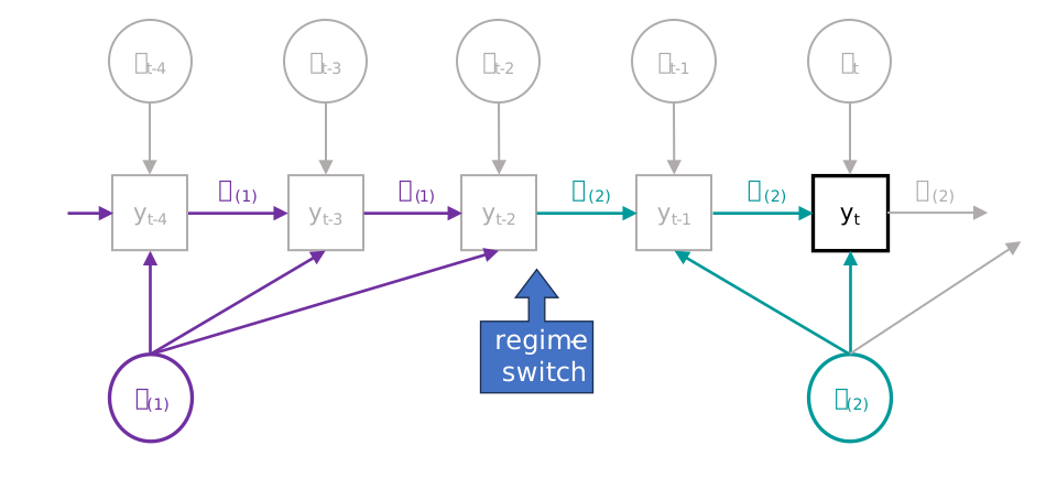
Making use again of the fact that the innovations do not contribute to the expectation, and that the infinite sum of indirect effects from \(c_{(1)}\) forms a geometric series, the expected value of \(y_t\) two occasions after the switch can be expressed as
\[E[y_t] = c_{(2)} + \phi_{(2)}c_{(2)} + \phi_{(2)}^2 \frac{c_{(1)}}{1-\phi_{(1)}}.\]
It shows that the effect of the long-run mean from the first regime is becoming less important, and that the effect of \(c_{(2)}\) is increasing.
3.4 When the switch took place between \(t-3\) and \(t-2\)
Similarly, you can derive the expectation three occasions after the switch. The visualization of this is given in Figure 4.
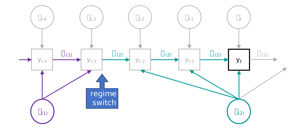
The expected value for \(y_t\) three occasions after the switch is
\[E[y_t] = c_{(2)} + \phi_{(2)}c_{(2)} + \phi_{(2)}^2 c_{(2)} + \phi_{(2)}^3 \frac{c_{(1)}}{1-\phi_{(1)}},\]
showing that the contribution of the long-run mean from the first regime has now further decreased, whereas the effect of \(c_{(2)}\) has further increased.
3.5 When the switch took place between \(t-4\) and \(t-3\)
Four occasions after the switch, the expectation is
\[E[y_t] = c_{(2)} + \phi_{(2)}c_{(2)} + \phi_{(2)}^2 c_{(2)} + \phi_{(2)}^3 c_{(2)} + \phi_{(2)}^4 \frac{c_{(1)}}{1-\phi_{(1)}},\]
which can be visualized as in Figure 5.
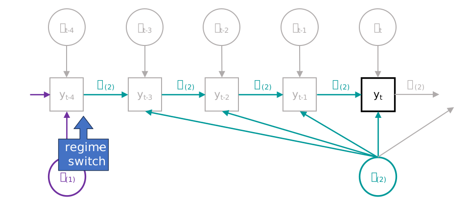
This approach can be used to investigate further what happens when the switch took place further in the past; but the expressions found above already reveal what the general pattern will be: With each additional time step away from a regime switch the contribution of the parameters of the second regime grows while the influence of the first regime diminishes.
3.6 Implied trajectory
The derivations above show a systematic pattern of what to expect for \(y_t\):
\(\frac{c_{(1)}}{1-\phi_{(1)}}\) before the switch
\(c_{(2)} + \phi_{(2)} \frac{c_{(1)}}{1-\phi_{(1)}}\) one occasion after the switch
\(c_{(2)} + \phi_{(2)}c_{(2)} + \phi_{(2)}^2 \frac{c_{(1)}}{1-\phi_{(1)}}\) two occasions after the switch
\(c_{(2)} + \phi_{(2)}c_{(2)} + \phi_{(2)}^2 c_{(2)} + \phi_{(2)}^3 \frac{c_{(1)}}{1-\phi_{(1)}}\) three occasions after the switch
\(c_{(2)} + \phi_{(2)}c_{(2)} + \phi_{(2)}^2 c_{(2)} + \phi_{(2)}^3 c_{(2)} + \phi_{(2)}^4 \frac{c_{(1)}}{1-\phi_{(1)}}\) four occasions after the switch
etc.
This shows that in the long run—and if the process remains in the second regime—the last term that contains the parameters associated with the first regime will go to zero (because the weight \(\phi_{(2)}^m\) goes towards zero as \(m\) grows). Furthermore, the part that depends on the parameters of the second regime will become an increasingly long expression that converges to
\[\frac{c_{(2)}}{1-\phi_{(2)}},\]
which forms the long-run mean of the second regime.
The expectations presented above form the underlying trajectory that gets the process from fluctuating around \(\mu_{(1)}=c_{(1)}/(1-\phi_{(1)})\) to fluctuating around the long-run mean of the second regime \(\mu_{(2)} = c_{(2)}/(1-\phi_{(2)})\). It is this underlying trajectory that is driving the series in red in Figure 1.
4 A minor model tweak with major consequences
Recall that in the second version of the regime-switching model, you have two long-run means: The long-run mean of the current regime (i.e., \(\mu_{(S_t)}\)), which is included as the intercept; and the long-run mean that the process was in at the previous occasion (i.e., \(\mu_{(S_{t-1})}\)), which is subtracted from the lagged predictor.
If you reformulate the model slightly, such that it includes as its predictor the deviation from the long-run mean of the current regime (i.e., \(y_{t-1} - \mu_{(S_t)}\)), rather than the deviation from the long-run mean of the regime the process was in at the previous occasion (i.e., \(y_{t-1} - \mu_{(S_{t-1})}\)), you get
\[y_t = \mu_{(S_t)} + \phi_{1(S_t)}(y_{t-1} - \mu_{(S_{t})}) + \epsilon_t .\]
This may seem like a minor adjustment; yet, this makes a huge difference in what happens right after the switch from one regime to another. In fact, this adjusted version results in a model that is identical to the model with intercepts and the lagged observed predictor (without subtracting any mean).
Consider the behaviors of the two models after the switch in Figure 1. The last observation prior to the switch is \(y_{20}=12.08\). Its deviation from the long-run mean of the regime the process was in at \(t=20\) is quite small: \(y_{20} - \mu_{(S_{20})}=12.08-10=2.08\). The value of this displacement does not require much time to wash out and vanish from the system, as shown by the blue series.
In contrast, if you determine how this score deviates from the long-run mean of the regime the process is in at occasion \(t=21\), you get a quite substantial deviation: \(y_{20} - \mu_{(S_{21})}= 12.0 -12.02\). This approach thus implies a large negative displacement from the long-run mean after the regime switch, and it takes time for the effect of this to wash out of the system, as is shown by the trajectory of the red series after \(t=20\). The trajectory towards the new equilibrium can be understood as an instance of displacement in an AR model.
5 Think more about
While the derivations presented above clearly show what you can expect when there is a single regime switch, things become more messy when there are recurrent and frequent switches. In that case, a process that is based on the first formulation (with the uncentered lagged predictors) may never reach the long-run equilibrium that characterizes a regime; this is illustrated in the article about Markov-switching autoregressive (MS-AR) modes. Also, the expected values and their implied trajectory for such processes will be much more complicated than the one derived above, where there was only one switch.
Hence, while the insights that these derivations provide you are helpful in understanding some of the complexities of regime-switching models, it is important to realize that further nuance arises when a process switches multiple times and more quickly. One particular regime-switching model for which this is relevant is the self-exciting threshold autoregressive (SETAR) model, which tends to switch back and forth quite frequently.
Another situation in which the trajectory from one regime to the other may be less clearly visible, is when the difference in long-run mean between the two regimes is not that large. In the example provided in Figure 1, the difference was quite substantial given the amount of variability within each regime. But when the difference in the long-run means is smaller, or similarly, when the variance within the regimes is larger, this trajectory becomes less prominent. Then the difference between these two formulations also becomes less relevant.
Finally, when interpreting the parameters of a model that allows for the gradual transition when a regime switch has taken place, you should keep in mind that what is referred to as the “long-run mean” of an intercept, may not represent the mean of the observations that fall in this regime. It is even possible that the long-run mean of a regime is never reached. This depends on the difference between the regimes, the amount of autoregression, and the speed with which transitions take place; you can investigate this with the tool provided in the article about the MS-AR model.
6 Takeaway
While the two formulations for a linear AR process–either based on having the observed variable as the lagged predictor, or having the mean-centered observed variable as the lagged predictor–are simple reparameterizations of each other, this equivalence breaks down in case there are regime switches. The crux of this difference lies in the fact that while the former formulation will result in displacement when the process switches regimes, the latter does not. The effect of displacement in an AR model is described in more detail in the article about the two formulations of an AR model.
When a regime-switching AR model is based on AR processes with the observed variable as the lagged predictor, the transition from one regime to another is more gradual. The trajectory towards the new long-run mean is governed by the degree of autoregression in the new regime. When the regime-switching AR model is based on AR processes with mean-centered observations as the lagged predictor (and the mean that is used for this is the mean from the regime the lagged predictor belonged to), then the transition is just about instant.
Hence, when you think the transition from one regime to another is somewhat gradual, it is more appropriate to use the former formulation. When, instead, you think the switch is instantaneous, the latter formulation is better suited. Most importantly, you should realize that the formulation can really make a difference here. However, in practice, it may not be that clear whether switches are gradual or instant; this depends also on how much overlap there is in the distributions implies by the different regimes.
7 Further reading
We have collected various topics for you to read more about below.
Acknowledgments
This work was supported by the European Research Council (ERC) Consolidator Grant awarded to E. L. Hamaker (ERC-2019-COG-865468).
References
Citation
@article{hamaker2026,
  author = {Hamaker, Ellen L. and Hoekstra, Ria H. A.},
  title = {Regime-Switching Autoregressive Model with Intercept Versus
    Mean},
  journal = {MATILDA Preprints},
  number = {2026-05-29},
  date = {2026-05-29},
  url = {https://matilda.fss.uu.nl/articles/ar-mean-vs-intercept-switch.html},
  langid = {en}
}