
Two formulations of an autoregressive model
This article is about multiple ways in which an autoregressive (AR) model can be expressed, and how the parameters of these expressions are related to each other. You can either use an AR formulation that includes an intercept \(c\), or a formulation that contains the mean of the process \(\mu\) as a parameter. These two formulations are mathematically equivalent, meaning they are reparameterizations of each other and the parameters of one can be expressed in terms of the parameters of the other.
This model equivalence may seem to suggest that it does not matter which formulation you use when analyzing your data. While this is true in terms of model fit, the two formulation result in different parameters, and knowing whether you have an estimate of \(c\) or of \(\mu\) is important for two reasons. First, it has consequences for how you should interpret the results from a substantive point of view; this becomes especially important when you are investigating individual differences in parameters of an AR model. Second, the equivalence does not hold when you are dealing with regime-switching AR models, in which the process is characterized by switches between two or more distinct AR processes over time. The current article focuses primarily on the first of these two reasons; however, you can also read it as a stepping stone towards understanding the second issue.
Below you can read more about: 1) the two traditional representations of an AR model; 2) how the two formulations are related; 3) what the difference is between the intercept and the mean of an AR model and how these should be interpreted; and 4) how to estimate the various formulations of an AR model.
1 Two representations of an AR model
In the time series literature, the AR model is typically represented in one of two ways: Either using a single equation in which the observed outcome is regressed on lagged versions of itself, or based on two separate equations that decompose the observed scores into a mean with autoregressive residuals. Both versions are presented below.
1.1 Single-equation representation with the intercept \(c\)
The most common way in the time series literature (e.g., Hamilton, 1994) to represent an AR model is with a single equation, that is,
\[y_t = c + \phi_1 y_{t-1} + \dots + \phi_p y_{t-p} + \epsilon_t.\]
It shows that the current score \(y_t\) is regressed on itself at preceding occasions, and there is a random, unpredictable component \(\epsilon_t\), which is referred to as the innovation, random shock, perturbation, or residual. The innovations form a white noise series over time, with a mean of zero and variance \(\sigma_{\epsilon}^2\).
The intercept \(c\) on the right-hand side enters the process recursively, because it is also part of past versions of \(y\); it is thus entangled in the dynamics of the process. To see this entanglement in more detail, consider the first-order autoregressive (AR(1)) model
\[y_t = c + \phi_1 y_{t-1} + \epsilon_t,\]
which is visualized as a path diagram in Figure 1.
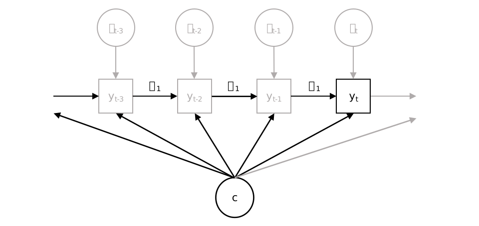
From this path diagram it becomes clear that the intercept \(c\) has a direct effect on \(y_t\), but that it also has indirect effects through past versions of \(y\), that is: \(\phi_1 c + \phi_1^2 c + \phi_1^3 c \dots\). This sum of indirect effects is infinite, meaning there is always another additional past term.
Yet, this does not mean that the sum results in an infinitely large number. When \(-1<\phi_1<1\) (which is a necessary constraint for an AR(1) process to be stationary), the indirect effects in this series become increasingly smaller as they concern a larger temporal distance: For instance, when \(\phi_1=0.5\), then \(\phi_1^2=0.25\)m and \(\phi_1^3=0.125\). In that case, the infinite series \((1 + \phi_1 + \phi_1^2 + \phi_1^3 + \phi_1^4 + \dots)\) is known to converge to \(1/(1-\phi_1)\); this follows from a standard result on geometric series (see for instance p.713 of Hamilton, 1994).
The intercept \(c\) from the expression above is sometimes interpreted to represent the mean of the process. However, this is incorrect; to get the mean \(\mu\), you can use a different formulation. or derive the mean from the intercept \(c\) and the autoregressive parameters using the result that is presented in following section.
1.2 Two-equation representation with the mean \(\mu\)
An alternative way to represent the AR model is through two separate equations that disentangle the mean of the process from its dynamics. The first equation in this formulation is
\[y_t = \mu + a_t,\] where \(\mu\) represents the long-run mean of the process, and \(a_t\) represents the temporal deviation from this mean, which can be referred to as the residual. A second equation is used in this formulation to specify an AR process for the residuals, that is
\[a_t = \phi_1 a_{t-1} + \dots + \phi_p a_{t-p} + \epsilon_t.\] Since these residuals—by definition—have a mean of zero (because the innovations \(\epsilon\) have a mean of zero), the current representation of an AR process can be described as a mean \(\mu\) with AR(\(p\)) residuals.
If you want to compare this two-equation expression to the one-equation formulation that was presented before, it is useful to consider the AR(1) model again, which has
\[a_t = \phi_1 a_{t-1} + \epsilon_t.\]
This formulation of the AR(1) model is visualized as a path diagram in Figure 2.
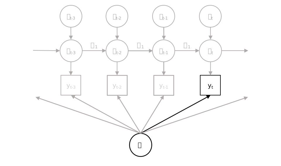
You can see that the parameter \(\mu\) only has a direct effect on \(y_t\): There are no indirect effects through past version of \(y\). This is because the dynamics are not modeled between the \(y\)’s, as was the case for the representation of the model in Figure 1, but between the residuals.
2 Connecting the two formulations of an AR(\(p\)) process
There are various ways to show how the two formulations of an AR model that were presented above are related (Hamilton, 1994). One of these is to start with the two-equation formulation and realizing that the lagged predictors in the second equation can be expressed as \(a_{t-1} = y_{t-1} - \mu\) up to \(a_{t-p} = y_{t-p} - \mu\). Using these as the predictors of \(a_t\) (i.e., in \(a_t = \phi_1 a_{t-1} + \dots + \phi_p a_{t-p} + \epsilon_t\)), and subsequently plugging that expression for \(a_t\) into \(y_t = \mu + a_t\), you can write
\[y_t = \mu + \phi_1 \bigl(y_{t-1} - \mu\bigr) + \dots + \phi_p (y_{t-p} - \mu) + \epsilon_t.\]
This shows that you can use a single-equation expression of the AR(\(p\)) model with an intercept that is actually identical to the mean \(\mu\): This is achieved by including the centered—rather than the raw—lagged predictors in the equation. (i.e., \(y_{t-1}-\mu\) rather than \(y_{t-1}\), etc.).
This latter expression helps to connect the intercept \(c\) from the initial formulation of an AR process to the mean \(\mu\) from the second formulation of the AR model. Below, this is first shown for an AR(1) process, and subsequently for an AR(\(p\)) process.
2.1 Mathematical connection between \(c\) and \(\mu\) in an AR(1) process
An AR(1) model can be expressed with the centered lagged observation as its predictor through
\[y_t = \mu + \phi_1 \bigl(y_{t-1} - \mu\bigr) + \epsilon_t.\]
Getting rid of the parentheses, you can write this as
\[y_t = \mu - \phi_1 \mu + \phi_1 y_{t-1} + \epsilon_t.\] Comparing the latter to the initial expression for an AR(1) (i.e., \(y_t = c + \phi_1 y_{t-1} + \epsilon_t\)), you can see that the intercept \(c\) can be expresses as a function of the mean \(\mu\) and the autoregressive parameter \(\phi_1\), through
\[c=(1-\phi_1)\mu\]
and thus
\[\mu = \frac{c}{1-\phi_1}.\]
This shows that when you have obtained \(c\) and \(\phi_1\) with the first formulation, you can derive \(\mu\); and vice versa, when you have obtained \(\mu\) and \(\phi_1\) you can derive \(c\).
2.2 Mathematical connection between \(c\) and \(\mu\) in an AR(\(p\)) process
In the more general case of an AR process of order \(p\), you can write
\[y_t = \mu + \phi_1 y_{t-1} - \phi_1 \mu +\dots + \phi_p y_{t-p} - \phi_p \mu +\epsilon_t.\]
By rearranging this so that all the terms with \(\mu\) are collected at the start, you get
\[y_t = \mu - \phi_1 \mu - \dots - \phi_p \mu + \phi_1 y_{t-1} +\dots + \phi_p y_{t-p} +\epsilon_t.\]
The part \(\mu - \phi_1\mu - \dots - \phi_p \mu = (1 -\phi_1 -\phi_2 -\dots -\phi_p)\mu\) is a constant which forms the intercept \(c\) in the first expression for the AR(\(p\)) model, that is
\[c = (1 - \phi_1 - \dots \phi_p) \mu.\] This also implies the reverse, that is
\[\mu = \frac{c}{1-\phi_1 -\dots-\phi_p}.\]
This shows how the mean \(\mu\) of an AR(\(p\)) process can be derived from the intercept \(c\) and the autoregressive parameters.
2.3 Conclusion
The above has shown that the crucial difference between the various formulations of an AR process is not whether you have one or two equations, but whether you use the observed variables as lagged predictors (e.g., \(y_{t-1}\)), or that you use the mean-centered observed variables as the lagged predictors (e.g., \(y_{t-1}-\mu\)). The latter is associated with obtaining an estimate of \(\mu\), whereas the former is related to obtaining an estimate of \(c\).
Given the mathematical difference between the intercept \(c\) and the mean \(\mu\), it becomes clear that there must be a difference in how you interpret these parameters from a substantive point of view. This is elaborated on in the next section.
3 Interpretation of intercept versus mean
The interpretation of the intercept \(c\) from an AR(\(p\)) model is the same as the interpretation of an intercept in any regression equation: It represents the expected (or predicted) value for the outcome variable when all predictors take on the value zero. In an AR process this means that all the \(p\) lagged versions of \(y_t\) should take on the value zero.
Below, you can see a more detailed explanation of this in the context of an AR(1) process, followed by an interactive tool that allows you to try out various parameter values for \(c\) and \(\phi_1\) of an AR(1) process to see how this affects \(\mu\). Subsequently, the result is extended to the general case of an AR model of order \(p\), followed by a brief discussion of whether to prefer the expression based on \(c\) or on \(\mu\).
3.1 Interpretation of the intercept in an AR(1) model
The intercept in an AR(1) model represents the expected value for \(y_t\) when \(y_{t-1}=0\). This can be visualized by plotting \(y_t\) against \(y_{t-1}\), and considering the regression line, which is \(\hat{y}_t = c + \phi_1 y_{t-1}\). An example of this is provided in Figure 3.
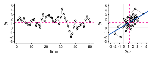
The time series in these plots were generated with an intercept of \(c=0.5\) and an autoregressive parameter of \(\phi_1=0.6\). In the left panel the sequence \(y_t\) is plotted against time for 50 occasions. The pink dashed line represents the long-run mean which is obtained from the intercept and autoregressive parameter through \(\mu =0.5/(1-0.6) = 1.25\).
In the right panel, \(y_t\) is plotted against itself at the preceding occasion \(y_{t-1}\), with the long-run mean plotted for both as dashed pink lines. The blue solid line represents the expected value for \(y_t\) given \(y_{t-1}\). The slope of this line is determined by the autoregressive parameter (i.e., \(\phi_1=0.6\)). This regression line crosses the vertical axis at the value 0.5: This is the expected value for the outcome \(y_t\) when the predictor \(y_{t-1}=0\). Importantly, this value does not correspond to the long-run mean \(\mu\), which represents the equilibrium of the process.
3.2 Interactive tool for the connection in an AR(1) model
To allow you to see how the intercept, autoregressive parameter, and mean of an AR(1) process are related, you can make use of the interactive tool below. It allows you to choose the intercept \(c\) and the autoregressive parameter \(\phi_1\). From these values the long-run mean \(\mu\) is computed. Furthermore, given a sequence of innovations \(\epsilon\) (with a mean of zero and a standard deviation of one), the sequence \(y\) is generated and plotted.
#| '!! shinylive warning !!': |
#|   shinylive does not work in self-contained HTML documents.
#|   Please set `embed-resources: false` in your metadata.
#| standalone: true
#| viewerHeight: 430
library(shiny)
library(bslib)

## file: app.R
library(shiny)
library(ggplot2)
library(patchwork)

# -------------------------
# Fixed settings
# -------------------------
N <- 50
BURNIN <- 100
axis_line_width <- 0.4

# -------------------------
# Build y from fixed residuals
# -------------------------
buildSeries <- function(e, c0, phi, n = N, burnin = BURNIN) {
  stopifnot(length(e) >= n + burnin)

  y <- numeric(n + burnin)
  for (t in 2:(n + burnin)) {
    y[t] <- c0 + phi * y[t - 1] + e[t]
  }

  y <- y[(burnin + 1):(burnin + n)]
  data.frame(y = y, t = seq_len(n))
}

# -------------------------
# Plotting
# -------------------------
plotTimeSeries <- function(dat, c0, phi) {

  dat$y_lag <- c(NA, dat$y[-length(dat$y)])
  y_breaks <- pretty(c(dat$y, 0))
  y_lim <- range(y_breaks)
  x_breaks <- pretty(dat$t)
  mu_theory <- c0 / (1 - phi)

  # ---- Scatter (RIGHT) ----

  p_ss <- ggplot(dat, aes(y_lag, y)) +
    geom_abline(intercept = c0, slope = phi,
                linewidth = 0.9, colour = "#0F52BA") +
    geom_vline(xintercept = mu_theory, linetype = 2,
               linewidth = 0.8, colour = "#EC008C") +
    geom_hline(yintercept = mu_theory, linetype = 2,
               linewidth = 0.8, colour = "#EC008C") +
    geom_point(size = 4, shape = 21, fill = "white", stroke=1.1, color = "black") +
    geom_vline(xintercept = 0, linewidth = 0.25) +
    geom_hline(yintercept = 0, linewidth = 0.25) +
    # add numbers along axes
    geom_text(data = data.frame(x = y_breaks),
              aes(x = x, y = 0, label = x),
              vjust = 1.6, size = 5) +
    geom_text(data = data.frame(y = y_breaks),
              aes(x = 0, y = y, label = y),
              hjust = 1.3, size = 5) +
    coord_cartesian(
      xlim = y_lim,
      ylim = y_lim
    ) +
    labs(x = bquote(y[t-1]), y = bquote(y[t])) +
    theme_void() +
    theme(
      text = element_text(size = 16),
      axis.title = element_text(size = 16),
      axis.text = element_blank()  # numbers now drawn manually
    )

  # ---- Time series (LEFT) ----
  p_ts <- ggplot(dat, aes(t, y)) +
    geom_hline(yintercept = mu_theory, linewidth = 0.8, colour = "#EC008C", lty=2) +
    geom_hline(yintercept = 0, linewidth = 0.25) +
    geom_line(linewidth = 0.75) +
    geom_point(size = 4, shape = 21, fill = "white", stroke=1.1, color = "black") +
    geom_segment(x = -Inf, xend = -Inf, y = y_lim[1], yend = y_lim[2],
                 linewidth = axis_line_width) +
    geom_segment(y = -Inf, yend = -Inf, x = min(x_breaks), xend = max(x_breaks),
                 linewidth = axis_line_width) +
    scale_x_continuous(breaks = x_breaks) +
    scale_y_continuous(breaks = y_breaks) +
    coord_cartesian(xlim = range(x_breaks), ylim = y_lim) +
    labs(x = "time", y = bquote(y[t])) +
    theme_void() +
    theme(
      text = element_text(size = 16),
      axis.text.x = element_text(margin = margin(6, 6, 6, 6)),
      axis.text.y = element_text(margin = margin(6, 6, 6, 6)),
      axis.title = element_text(size = 16)
    )

  p_ts + p_ss + plot_layout(widths = c(2, 1))
}

# -------------------------
# UI
# -------------------------

ui <- fluidPage(
  fluidRow(
    column(
      4,
      numericInput(
        "c0",
        label = HTML("<h4>Intercept c</h4>"),
        value = 0.4, step = 0.1
      )
    ),

    column(
      4,
      sliderInput(
        "phi",
        label = HTML("<h4>Autoregression \u03D5<sub>1</sub></h4>"),
        min = -0.99, max = 0.99,
        value = 0.6, step = 0.05
      )
    ),

    column(
      4,
      style = "padding-top: 6px;",  # <-- move entire column content down
      withMathJax(),
      uiOutput("mu_val")   # <- only this
    )
  ),

  actionButton("refresh", "Refresh"),

  plotOutput("main_plot", height = "260px")
)

# -------------------------
# Server
# -------------------------
server <- function(input, output) {

  # fixed residuals
  e_vals <- reactiveVal(rnorm(N + BURNIN, sd = 1))

  observeEvent(input$refresh, {
    e_vals(rnorm(N + BURNIN, sd = 1))
  })

  dat <- reactive({
    buildSeries(e_vals(), input$c0, input$phi)
  })

  output$main_plot <- renderPlot({
    plotTimeSeries(dat(), input$c0, input$phi)
  })

  # Compute mu dynamically for UI
  output$mu_val <- renderUI({
    mu <- input$c0 / (1 - input$phi)

    # Line 1: plain text
    # Line 2: MathJax display math with fraction
    tagList(
      div("Computed mean μ", style = "font-size:18px; font-weight:400;"),
      # proper MathJax equation
      div(
        style = "font-size:16px;",   # <-- only this div’s font size
        withMathJax(),
        paste0("$$\\mu = \\frac{c}{1-\\phi_1} = ", round(mu, 3), "$$")
      )
    )
  })
}

shinyApp(ui, server)
On the left, it shows the sequence plotted against time. The pink dashed line represents the long-run theoretical mean \(\mu\). In the right panel, each score \(y_t\) is plotted against the preceding score \(y_{t-1}\). The horizontal and vertical dashed pink lines represent the mean \(\mu\). The blue solid line represents the regression line based on the predictable part of \(y_t\), that is \(c + \phi_1 y_{t-1}\): Its intercept (where it crosses the vertical axis) is thus \(c\), and its slope is autoregressive parameter \(\phi_1\).
You can change the intercept and autoregressive parameter, while the sequence of innovations remains the same. The autoregressive parameter is constrained to lie between -1 and 1 to ensure stationarity (the tool allows values from -0.99 to 0.99). The intercept \(c\) can also be negative or positive, and is not constrained. When you set \(c\) to a value far enough from zero, you will get a scenario in which the intercept falls outside of the range of observed values for \(y\).
If you want a new version of the same model, you can press the refresh button: This results in a new sample of innovations \(\epsilon_t\) from a white noise process.
3.3 Generalizing the interpretation to an AR(\(p\)) process
To consider the intercept from an AR(2) process in a similar visual way as the intercept of an AR(1) process, you have to extend the two-dimensional plot of \(y_t\) against \(y_{t-1}\) to a three-dimensional plot of \(y_t\) against \(y_{t-1}\) and \(y_{t-2}\). The predictable part of \(y_t\) is now not just a line in a two-dimensional space, but actually a plane in a three-dimensional space. The intercept \(c\) now represents the value at which this plane crosses the vertical axis formed by \(y_t\).
For AR processes with \(p>2\) it becomes impossible to use this visualization as it involves more than three dimensions. But the interpretation of the intercept \(c\) remains the same: It is the value you should expect for \(y_t\) when all \(p\) lagged versions of \(y_t\) take on the value zero. In contrast, \(\mu\) represents the value you should expect for \(y_t\) when all \(p\) lagged versions of the outcome are equal to \(\mu\).
3.4 Preferring the mean \(\mu\) or the intercept \(c\)
There may be specific scenarios when the intercept \(c\) represents a meaningful quantity, but typically it will not really be of interest from a substantive point of view. There are even scenarios in which it is impossible to obtain a value of zero on the variable you are modeling: In that case, finding the expected value for \(y_t\) given \(y_{t-1}=0\) (and additional lagged versions of \(y_t\) when \(p>1\)) becomes a rather meaningless quantity from a substantive point of view.
Unnur has measured daily positive affect in a person for 60 days with ten items using a Likert scale from 1 to 5 for each item. She has decided to obtain the sum score across all ten items to represent a person’s overall positive affect: The resulting sum score thus has a theoretical range from 10 to 50.
Unnur decides to fit a first-order autoregressive model. When seeing the intercept, she at first thinks this should represent the person’s average score across the 60 days. But then she notices that the value of the intercept is 18, which she considers to be rather low given the possible range of sum score she uses. Moreover, the sample mean is actually 33. Unnur then realizes that the value 18 is the expected sum score for positive affect, when the sum score at the preceding day would be zero; this is something that is not possible, given the scale’s lower end of 10.
Unnur sees that, while it is important to estimate the intercept, it is not of substantive interest. She would rather obtain an estimate of the mean instead. She can either compute the mean from the estimates of the intercept and autoregressive parameter, but this will not give her any insight in the uncertainty of the estimated mean. She therefore concludes that it is best to make use of an estimation procedure based on the state-space model and the Kalman filter, as this will allow her to specify the model as a mean with AR(1) residuals.
In contrast, the mean will typically be of interest, because it represents the long-run equilibrium that characterizes the process over time. You can think of it as the attractor of the system: It is the value towards which the process is inclined to return when no external shocks are given to the system.
4 Estimation
If you want to estimate the parameters of an AR(\(p\)) model, you can use a representation that includes \(c\) or one that includes \(\mu\). These should result in the same point estimates for the autoregressive coefficients and the innovation variance. For interpretation of the results, it is important that you know whether you have obtained an estimate of the intercept \(c\), or of the mean \(\mu\).
When using existing software packages, you are probably restricted to using one or the other. However, when you make use of a Kalman filter, both versions of an AR model can be specified. This stems from the fact that formulating an AR model in state-space format allows you to: a) use the measurement equation to separate the mean from the residuals which are modeled as an AR process with the transition equation; or b) only use the transition equation to specify the entangled one-equation version of an AR model and estimate its intercept and AR coefficients.
While the mathematical derivations shown in this article imply that these two model specifications should result in the exact same autoregressive parameters and innovation variance, in practice the equivalence may break down due to differences in initiating the Kalman filter. Such differences are likely to be accompanied by differences in model fit. The latter should be considered an anomaly rather than a meaningful difference between the model formulations. Further differences in estimation may arise when you take a Bayesian approach, where prior distributions may not support the model equivalence.
Unnar wants to use a Kalman filter to get an estimate of her participant’s long-run mean \(\mu\) and their autoregression \(\phi_1\) based on their daily positive affect measurements. For this, Unnar needs to initiate the Kalman filter by defining the state of the underlying state-space model at occasion \(t=0\). Unnar knows that often people specify this to be zero, but that this is not necessarily a realistic value for the initial state.
To get a better understanding of this issue, Unnar decides to write down carefully the model in terms of the state-space equations, to get a thorough understanding of what the initial state is supposed to represent. In particular, she wants to know whether this should represent the outcome prior to when the observations started (i.e., \(y_0\)), or that it should represent the deviation of the unobserved outcome prior to when the observations started from the long-run theoretical mean (i.e., \(y_0 - \mu\)).
Unnar concludes that if she uses the specification of an AR(1) model that results in an estimate of \(\mu\) rather than \(c\), the initial state should represent the deviation of \(y_0\) from the long-run mean; then, choosing zero to initiate the filter does not seem a bad idea. But based on the MATILDA article about displacement of an AR process, Unnar realizes that even in this case zero is not necessarily a good value: If she sees reason to believe that the process started far away from its long-run equilibrium \(\mu\), then it may be better to choose a value for the initial state that represents such a discrepancy.
Instead of using a Kalman filter approach for estimating the parameters of an AR process, you may also consider using ordinary least squares estimation. When there are no missing observations, you can simply include lagged versions of the outcome as observed predictors in a regression analysis. This way you can get estimates of the intercept \(c\) and the autoregressive parameters, which you can then use to obtain an estimate for the long-run mean \(\mu\).
To obtain a direct estimate of the long-run mean \(\mu\) with this approach, you may decide to use sample mean centering of the lagged predictors. While this makes sense from the derived relations presented above, in practice it will not always work well: Especially when the series are short and/or when there is displacement of the process, there can be a considerable discrepancy between the sample mean and the long-run theoretical mean \(\mu\). Therefore, using an estimation approach that is based on a Kalman filter would be better, although—as pointed out above—its initiation may pose a challenge.
5 Think more about
In this article you have seen that the two model formulations for an AR process are equivalent: This means they can give rise to the exact same data, and can thus also equally well describe observed data. The equivalence generalizes to the autoregressive moving-average (ARMA) process; since the moving-average part by definition does not involve any components with non-zero means, its presence or absence has no bearing on the mean structure. Hence, the results for an AR(\(p\)) model can also be applied to an ARMA(\(p\),\(q\)) model.
The equivalence between model specification also generalizes to multivariate versions like a [vector autoregressive (VAR)] model, or a [vector autoregressive moving-average (VARMA) model]. In these cases there is a vector of intercepts that can be connected to a vector of means; the exact relation is based on matrix algebra (see Hamilton, 1994).
This may give you the impression that it does not matter whether you formulate an AR-based model with a mean or with an intercept. However, there are extensions for which this equivalence does not hold up.
One class of such extensions are regime-switching models based on AR models. In regime-switching models, the process alternates between two or more data generating mechanisms, each of which is an AR (or AR-based) model. Examples are the Markov-switching autoregressive (MS-AR) model and the threshold autoregressive (TAR) model. The behavior of regime-switching AR models depends critically on whether a formulation with intercepts or means per regime are used; you can read more about this in the article about the regime-switching AR model with intercept versus mean.
Another class of extensions is formed by adding an exogenous variable to the AR model. This can also be done in various ways: Either in the single expression with an intercept, or in a version which forms a regular regression model but with AR residuals. These two options are known as the autoregressive moving-average model with exogenous inputs (i.e., the ARMAX model), and dynamic regression respectively. Just as with the constant in an AR model, the place where the exogenous variable enters the model determines the way in which it affects the trajectory of the process; to understand how this works, it helps if you first understand how the two versions of an AR formulation are connected, as explained in the current article.
One particular version of this latter extension is when time \(t\) is included as an exogenous input. Here you have the choice again to include it in the entangled equation that also contains the lagged versions of the outcome, meaning time will have both direct and indirect effects, or to have a trend disentangled from its autoregressive residuals, meaning time only has a direct effect on the outcome. You can read more about this in the article about trend and autoregression.
6 Takeaway
To correctly interpret the parameters of your AR model, it is important to understand their role in the process. An intercept has quite a distinct role from that of a mean, and confusing one for the other would imply your conclusions are misinformed. Therefore, knowing the difference between the two ways to represent an AR process and being able to recognize which version was implemented in the software you use or in the article you are reading, is critical.
It is also good to realize that the two formulations are simple reparameterizations of the same model. This means that the two formulations can give rise to the exact same time series, and that fitting the two versions to empirical data will result in the exact same model fit. The autoregressive parameters and innovation variance of the two formulations are identical, so that when your focus is on these parameters, it makes no difference which formulation you use. However, some differences in model fit and parameter estimates may arise from using different ways to initiate the Kalman filter to estimate the model, and/or prior distributions when Bayesian estimation is used. Such differences tend to become smaller for longer time series.
Most software packages that allow for \(N=1\) time series analysis probably make use of the formulation with an intercept, rather than with the long-run mean. Yet, from a substantive perspective, the long-run mean is probably more interesting than the intercept. In that case, the intercept together with the autoregressive parameters can be used to derive the value of the long-run mean. The long-run mean that is implied by the underlying process can differ considerably from the sample mean, due to large momentary deviations, especially when series are short and when there is displacement.
7 Further reading
We have collected various topics for you to read more about below.
- [Vector autoregressive (VAR) models]
- [Vector autoregressive moving average (VARMA) models]
- [Latent VAR models]
- [Multilevel AR models]
- [Dynamic structural equation modeling]
- [Replicated time series analysis]
Acknowledgments
This work was supported by the European Research Council (ERC) Consolidator Grant awarded to E. L. Hamaker (ERC-2019-COG-865468).
References
Citation
@article{hamaker2026,
  author = {Hamaker, Ellen L. and Hoekstra, Ria H. A.},
  title = {Two Formulations of an Autoregressive Model},
  journal = {MATILDA Preprints},
  number = {2026-05-29},
  date = {2026-05-29},
  url = {https://matilda.fss.uu.nl/articles/two-formulations-ar-model.html},
  langid = {en}
}