
Autoregressive model with displacement
This article is about the effect of displacement on the trajectory of an autoregressive (AR) process. Displacement implies that the process has been moved away from its long-run mean and outside the usual range of scores that can be expected based on its stationary distribution. Although the underlying data generating mechanism may be stationary, displacement can introduce temporary trajectories that resemble growth, decline, recovery, or adaptation. Understanding this phenomenon is important for interpreting short time series, recovery after shocks, interventions, and regime switches.
This article also helps clarify an apparent paradox that arises when comparing two other MATILDA articles: 1) the article on the two formulations of an AR model, which shows that an AR model formulation with an intercept is mathematically equivalent to an AR model formulation with a mean; and 2) the article about regime-switching AR models, which shows that an AR model formulation with an intercept results in different behavior following a regime switch than an AR model formulated with a mean. To understand why this happens it is important to understand how displacement propagates through an AR process.
Below you find: 1) a brief recap of the two ways in which an AR model can be represented; 2) a derivation of the stationary distribution of an AR model; 3) a numerical example that shows what happens when the process is displaced; 4) an interactive tool that allows you to try out the effect of displacement and how this interacts with other model characteristics; and 5) some implications this for estimating an AR model.
1 Various ways to express an AR(\(p\)) model
For a more in-depth treatment of AR models you can read the article on AR models and on the two formulations of an AR model. Here a brief recap for the current purpose of discussing displacement is provided.
There are various ways in which an AR model can be represented. In the time series literature (e.g., Hamilton, 1994), the most common formulation is
\[y_t = c + \phi_1 y_{t-1} + \dots + \phi_p y_{t-p} + \epsilon_t,\]
showing how \(y_t\) is regressed on—and perhaps shaped by—past versions of itself going back \(p\) steps in time. The term \(\epsilon_t\) is the unpredictable part, referred to as random shock, innovation, or perturbation, which is often assumed to come from a normal distribution; it has a mean of zero over time, and is a white noise process.
The parameter \(c\) is the intercept, which should not be confused with the mean of \(y\); it does not represent the long-run expectation for the outcome (that is, the value you would get if the random shocks would all be zero over time), but rather the expected value for the outcome \(y_t\) when all the predictors (i.e., the lagged versions of \(y\)) take on the value zero.
In the article about two formulations of an AR model, an alternative formulation of an AR model is presented, that is
\(\;\;\;\;\;\;\;\;\;\;\;\;\;\; y_t = \mu + a_t\)
\(\;\;\;\;\;\;\;\;\;\;\;\;\;\; a_t = \phi_1 a_{t-1} + \dots + \phi_p y_{t-p} + \epsilon_t.\)
The expression for \(a_t\) can be plugged into the expression for \(y_t\), which gives
\(\;\;\;\;\;\;\;\;\;\;\;\;\;\; y_t = \mu + \phi_1 a_{t-1} + \dots + \phi_p y_{t-p} + \epsilon_t.\)
Replacing the lagged versions of \(a\) in the latter expression by their expressions as deviations from the long-run mean \(\mu\) (i.e., \(a_{t-1} = y_{t-1} - \mu\) etc.), results in
\(\;\;\;\;\;\;\;\;\;\;\;\;\;\; y_t = \mu + \phi_1 (y_{t-1} - \mu) + \dots + \phi_p (y_{t-p} - \mu) + \epsilon_t.\)
This shows that the major difference is not whether the AR model is expressed with one or two equations, but whether the predictors that are included are lagged versions of the observed variable (i.e., \(y_{t-1}\) to \(y_{t-p}\)), or that these are lagged versions of the observed deviations from the long-run mean (i.e., \(y_{t-1}-\mu\) to \(y_{t-p}-\mu\)).
2 Stationary distribution of an AR(\(p\)) process
AR processes are by definition stationary; this implies that the autoregressive parameters \(\phi_1\) to \(\phi_p\) are bounded by specific constraints. When these stationarity constraints are in place, this implies that the long-run behavior of an AR process can be determined, based on its parameters. Here you can see how the long-run mean of an AR process can be derived using the first formulation of an AR process that was presented above, and how the long-run variance can be derived. With these two, it becomes possible to consider when a process is displaced.
2.1 Deriving the long-run mean
To obtain the long-run mean of an AR process based on the first model expression presented above, you can make use of the derivation that is quite often shown in the time series literature (e.g., Hamilton, 1994). It starts with taking the expected value on both sides, that is,
\[ E[y_t] = E[c + \phi_1 y_{t-1} + \dots + \phi_p y_{t-p} + \epsilon_t].\] Since the expectation of a sum can also be expresses as a sum of expectations, the right-hand side can be rewritten as
\[ E[y_t] = E[c] + E[\phi_1 y_{t-1}] + \dots E[\phi_p y_{t-p}] + E[\epsilon_t].\]
The expectation of the innovation \(\epsilon_t\) is zero, because the mean of the innovations is by definition zero. Hence, the last term on the right-hand side can be dropped from the expression.
Moreover, the autoregressive parameters \(\phi_1\) to \(\phi_p\) included in the middle terms on the right-hand side are constants and can be taken outside their respective expectations, and the expectation \(c\) is simply equal to \(c\) (because it is a constant). Together, this give
\[ E[y_t] = c + \phi_1 E[y_{t-1}] + \dots \phi_p E[y_{t-p}].\]
This is where the assumption of stationarity comes in: If you assume that the mean of \(y\) does not change over time, this can be expressed as
\[ E[y_t] =E[y_{t-1}]=\dots = E[y_{t-p}]=\mu.\]
Hence, you can replace all the expectations with \(\mu\) and write
\[\mu = c + \phi_1 \mu + \dots + \phi_p \mu.\]
Subsequently, moving all the \(\mu\)’s to the left gives
\[ \mu - \phi_1 \mu - \dots - \phi_p \mu= c\] which can be written as
\[ (1 - \phi_1 - \dots - \phi_p) \mu= c.\]
If you now divide both sides by \((1 - \phi_1 - \dots - \phi_p)\), this results in
\[ \mu = \frac{c}{1 - \phi_1 - \dots - \phi_p}.\]
The latter shows you how the mean that characterizes a stationary AR(\(p\)) process can be expressed as a function of the intercept \(c\) and the autoregressive parameters \(\phi_1\) to \(\phi_p\).
2.2 Deriving the long-run variance
If you want to derive the variance of an AR(\(p\)) process, this is somewhat more complicated than finding an expression for the mean: It requires either the use of matrix algebra, or something that is known as the Yule-Walker equations (see for instance p.59 in Hamilton, 1994).
But for an AR(1) process, it is relatively easy to derive the expression of the total variance. Looking at the AR model as a linear regression, you can write its variance as
\[Var(y_t) = \phi_1^2 Var(y_{t-1}) + Var(\epsilon_t).\]
Because the process is stationary, you can write \(Var(y_t) = Var(y_{t-1}) = \sigma^2_y\), and \(Var(\epsilon_t)=\sigma^2_{\epsilon}\), to get
\[\sigma^2_y = \phi_1^2 \sigma^2_y + \sigma^2_{\epsilon}.\]
Taking the first term on the right-hand side to the left gives
\[\sigma^2_y - \phi_1^2 \sigma^2_y = \sigma^2_{\epsilon},\]
which can also be expressed as
\[ (1 - \phi_1^2) \sigma^2_y = \sigma^2_{\epsilon}.\]
Dividing both sides by \((1 - \phi_1^2)\) results in
\[ \sigma^2_y = \frac{\sigma^2_{\epsilon}}{1 - \phi_1^2 }.\]
The expression for the long-run variance of an AR(2) process in terms of autoregressive parameters and the innovation variance is presented in the article about AR models; it shows this is already a much more complicated expression. This complexity increases as the order \(p\) increases, but the general point remains the same: Given stationarity, the long-run behavior of an AR process can be derived by expressing its stationary distribution in terms of the long-run mean and variance, which can be written as functions of the parameters of the process.
2.3 Deriving the long-run distribution
Typically, the innovations \(\epsilon\) are assumed to come from a normal distribution. In that case the stationary distribution of \(y\) is also a normal distribution. This implies that the stationary distribution of \(y\) is determined by the long-run mean and the long-run variance, that is, \(y \sim N(\mu, \sigma_y^2)\).
3 Numerical example of an AR(1) process with displacement
Using the stationary distribution, you can determine what range of scores can be expected for \(y\). For instance, when \(y\) has a normal distribution, you can say that 95% of the scores is expected to fall in between \(\mu - 1.96\sigma_y\) and \(\mu + 1.96\sigma_y\).
When a value falls outside this range, you may consider this an instance of displacement of the process: From a dynamic systems point of view, you would say the system has been moved far way from its attractor or equilibrium state. The dynamics of the system then determine its trajectory back to equilibrium. To see how such displacement operates through the two formulations of an AR model, it helps to look at a specific numerical example and compare the temporal trajectories that the two formulations imply.
3.1 Generating data using the AR expression with the intercept \(c\)
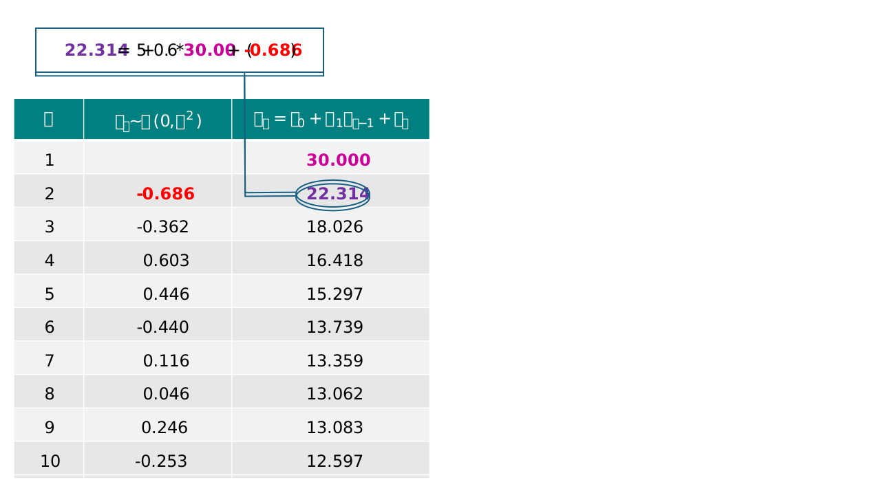
First, a short sequence of innovations was generated (for \(t=2, \dots, 10\)), which is included in the middle column of Figure 1. With these innovations, an AR(1) process was generated based on the single equation formulation with an intercept of \(c=5\), an autoregressive parameter of \(\phi_1=0.6\), and an innovation variance of \(\sigma^2=1\). These parameter values imply that the long-run mean is \(\mu=5/(1-0.6) = 12.5\), and the long-run variance of \(y\) is \(\sigma_{y}^2 = 1/(1-0.6^2)=1.5625\). The first occasion was set to \(y_1=30\), which is quite extreme given the long-run mean and variance of \(y\). The result of this is included in the last column of Figure 1.
The process that is created in this way is visualized in Figure 2. It also contains the long-run mean as the dashed pink line, and the shaded pink area represents the range within which 95% of the data points of this process are expected to fall when it has reached its long-run stationary state (i.e., based on \(\mu \pm 1.96\sigma_y\)). It visualizes clearly that the process starts far away from the range that is expected in the long-run, and it also shows that it takes some time before the process has reached the expected range given the stationary distribution.
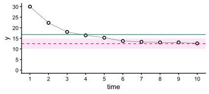
The plot also contains the sample mean as the solid green line. You can see that this not only deviates from the long-run mean \(\mu\), but that it actually falls outside the range that is to be expected for the observations themselves. This is the result of having an extreme starting value for the AR process and only observing this for a small number of occasions.
3.2 Generating data using the AR expression with the long-run mean \(\mu\)
To see whether the alternative representation of an AR model that involves the stationary mean \(\mu\) rather than the intercept \(c\) results in the same series, you can check the two columns that are added in Figure 3: The first of these contains \(a_t = \phi_1 a_{t-1} + \epsilon_t\), and the second contains \(y_t = \mu + a_t\). For \(t=1\), \(a_1\) was set to \(y_1 - \mu\) to start the process.
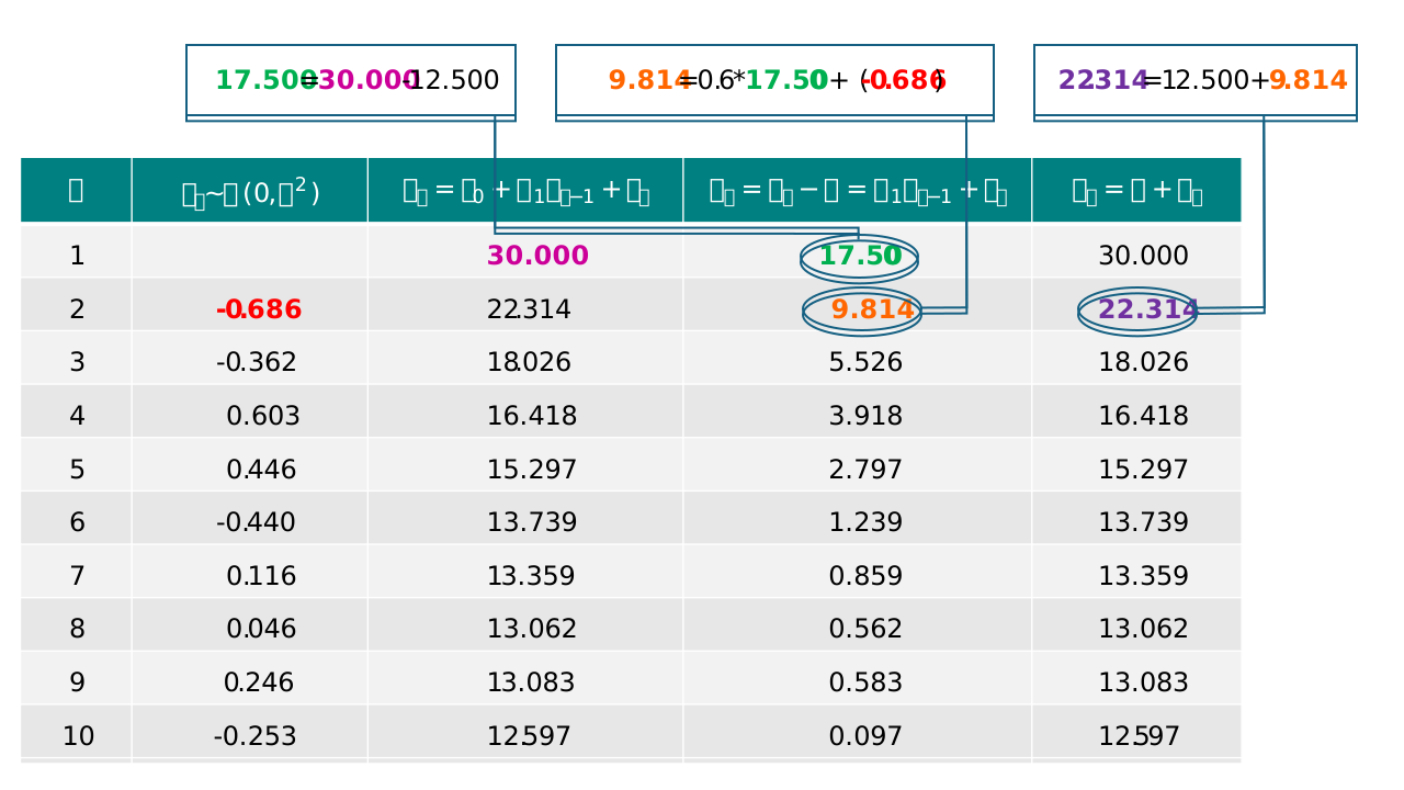
It shows that the two-equation representation with \(\mu\) results in the exact same numerical series as the one-equation representation with \(c\).
4 Interactive tool showing the effect of large displacements
You can obtain some intuition about the phenomenon described above with the tool presented here. It allows you to vary the intercept \(c\), the autoregression \(\phi_1\), the innovation variance \(\sigma_{\epsilon}^2\), the number of time points, and the initial value for \(y\).
On the right you see the data generating model based on the intercept, autoregression and innovation variance, as well as the model implied long-run mean \(\mu\) and variance \(\sigma^2_{y}\). When you change the intercept \(c\) and/or the autoregression \(\phi_1\), this long-run mean changes accordingly. Changing the autoregression \(\phi_1\) and/or the innovation variance \(\sigma_{\epsilon}^2\) results in a change in the variance of the process \(\sigma_{y}^2\).
#| '!! shinylive warning !!': |
#| shinylive does not work in self-contained HTML documents.
#| Please set `embed-resources: false` in your metadata.
#| standalone: true
#| viewerHeight: 630
library(shiny)
library(bslib)
## file: app.R
library(shiny)
library(ggplot2)
ui <- fluidPage(
# ---- CSS for grey refresh button ----
tags$head(
tags$style(HTML("
.btn-refresh {
background-color: #e5e5e5;
border-color: #bdbdbd;
color: #000;
}
.btn-refresh:hover {
background-color: #cccccc;
border-color: #999999;
color: #000;
}
"))
),
# ---- Two-column layout ----
fluidRow(
# Left column: Inputs
column(
width = 4,
#br(),
numericInput("c", label = HTML("<h4>Intercept c</h4>"), value = 2, step = 0.1),
sliderInput("phi", label = HTML("<h4>Autoregression \u03D5<sub>1</sub></h4>"), min = -0.999, max = 0.999, value = 0.5, step = 0.05),
numericInput("var_eps", label = HTML("<h4>Variance σ<sup>2</sup><sub style='position: relative; left: -0.4em;'>ϵ</sub></h4>"), value = 1, min = 0.0001, step = 0.1),
numericInput("n", label = HTML("<h4>Number of time points</h4>"), value = 15, min = 2, step = 1),
numericInput("y1", label = HTML("<h4>Initial value y<sub>1</sub></h4>"), value= -5, step = 0.5),
br(),
actionButton("refresh", "Refresh")
),
# Right column: Equation + plot
column(
width = 8,
HTML("<h4>Data generating model:</h4>"),
br(),
withMathJax(uiOutput("ar_eq")),
br(),
withMathJax(),
uiOutput("mu_val"), # <- only this
br(),
plotOutput("ts_plot", height = "350px")
)
)
)
server <- function(input, output, session) {
# ---- Standardized residuals ----
z_vals <- reactiveVal()
# Initialize residuals at startup
observe({
z_vals(rnorm(input$n))
})
# Regenerate residuals on Refresh button
observeEvent(input$refresh, {
z_vals(rnorm(input$n))
})
# Regenerate residuals if n changes
observeEvent(input$n, {
z_vals(rnorm(input$n))
}, ignoreInit = TRUE)
# ---- Simulate AR(1) ----
ts_data <- reactive({
n <- input$n
c <- input$c
phi <- input$phi
sigma <- sqrt(input$var_eps)
z <- z_vals()
req(length(z) >= n)
eps <- sigma * z[1:n]
y <- numeric(n)
y[1] <- input$y1
for (t in 2:n) {
y[t] <- c + phi * y[t - 1] + eps[t - 1]
}
data.frame(
t = 1:n,
y = y
)
})
# ---- Render AR(1) equation with parameter values ----
output$ar_eq <- renderUI({
c <- input$c
phi <- input$phi
var_eps <- input$var_eps
# Wrap the HTML string in withMathJax to ensure proper rendering
withMathJax(
helpText(
paste0(
"$$\\large y_t = ", round(c, 2),
" + ", round(phi, 2), " y_{t-1} + \\epsilon_t, \\quad \\quad \\epsilon_t \\sim N(0, ",
round(var_eps, 2), ") $$"
)
)
)
})
# Compute mu dynamically for UI
output$mu_val <- renderUI({
mu <- input$c / (1 - input$phi)
vary <- input$var_eps / (1 - input$phi^2)
# Line 1: plain text
# Line 2: MathJax display math with fraction
tagList(
div("Computed long-run mean and variance:", style = "font-size:18px; font-weight:400;"),
# proper MathJax equation
div(
style = "font-size:16px;", # <-- only this div’s font size
withMathJax(),
paste0(
"$$",
"\\mu = \\frac{c}{1-\\phi_1} = ", round(mu, 3),
#"\\\\[6pt]", # line break with spacing
"\\hspace{4em}",
"\\sigma_y^2 = \\frac{\\sigma_{\\epsilon}^2}{1-\\phi_1^2} = ", round(vary, 3),
"$$"
)
)
)
})
# ---- Plot ----
output$ts_plot <- renderPlot({
df <- ts_data()
c <- input$c
phi <- input$phi
var <- input$var_eps
vary <- var/(1-phi^2)
sdy <- sqrt(vary)
mu <- c/(1-phi)
sample.mean <- mean(df$y)
up95 <- mu + 1.96*sdy
lo95 <- mu - 1.96*sdy
ggplot(df, aes(x = t)) +
annotate(
"rect",
xmin = -Inf, xmax = Inf,
ymin = lo95, ymax = up95,
alpha = 0.1,
fill = "#EC009C"
) +
geom_hline(
yintercept = mu,
linetype = 2,
color = "#EC009C",
linewidth = 0.6
) +
geom_hline(
yintercept = sample.mean,
linewidth = 0.6, colour = "#14856d", lty=1
) +
geom_line(aes(y = y), color = "black", linewidth = 0.75) +
geom_point(
aes(y = y),
shape = 21,
fill = "white",
color = "black",
size = 3,
stroke = 1
) +
labs(
x = "time",
y = expression(y[t]),
title = "AR(1) process with sample mean and long-run mean"
) +
scale_x_continuous(breaks = seq(1, max(df$t), by = 1)) +
theme_minimal() +
theme(
panel.grid = element_blank(),
axis.text = element_text(size = 10),
axis.title = element_text(size = 10),
axis.line = element_line(linewidth = 0.8),
plot.title = element_text(size = 12),
axis.ticks = element_line(linewidth = 0.8),
axis.ticks.length = unit(4, "pt")
)
}, res = 120)
}
shinyApp(ui, server)
On the right you also see a simulated series based on the settings you specified. It includes the theoretical long-run mean \(\mu\) as the dashed pink line, and a shaded pink area that represents the range within which 95% of the data points of this process are expected to fall given its long-run stationary distribution.
In addition, you also see the solid green line that represents the sample mean based on the simulated data points. By changing \(c\) or \(\phi_1\), you can see how this changes both the sample mean and the long-run mean; the series of innovations (i.e., \(\epsilon_t\)) are kept constant when you change these parameters, allowing you to see very precisely how different parameter values changes the shape of the trajectory of the process towards its long-run equilibrium. By pressing the refresh button, a new series of innovations is generated, allowing you to see a different series generated from the same model settings.
To see how the autoregressive parameter \(\phi_1\) changes the trajectory of the series towards the long-run mean, you may first change this to \(\phi_1 = 0.9\); you will see that the process is still far from reaching its equilibrium state after 15 occasions, and also that the sample mean and the long-run mean are quite different. In contrast, if you change the autoregression to 0, this shows that the discrepancy between the sample mean and the long-run mean becomes almost negligible, and that the process is immediately in its stationarity range after the initial time point.
Additionally, you can also investigate what happens when you change the initial displacement \(y_1\), by increasing or decreasing it; again, the tool keeps the innovations constant, such that you can see the isolated effect of the initial value. It shows that when you have a (considerable) displacement in the negative direction (i.e., \(y_1 < \mu\)), the sample mean will be smaller than the long-run mean; in contrast, when the displacement is in the positive direction (i.e, \(y_1 > \mu\)), the sample mean will be larger than the long-run mean.
Furthermore, you can also change the intercept and/or the innovation variance and see how this affects the appearance of the series. Finally, you can investigate what happens when the number of time points is increased (this always results in a new sample of innovations). For instance, by setting the number of time points to 50, you can see it takes quite long to reach the stationarity range when the autoregressive parameter is \(\phi_1=0.9\); by using the refresh button, you can also see that this is highly dependent on the sample, which is a characteristic of having such an autoregressive parameter close to the stationarity bounds.
The long-run mean \(\mu\) is not necessarily close to the sample mean of a finite observed series. When there is large displacement at the start of the series (or when there is a major shock given to the system at a later occasion, moving the process far away from equilibrium), then the sample mean will deviate considerably from the long-run model implied mean. This difference is especially prominent when there is a lot of autoregression, and when the series are short.
5 Estimation
As discussed in the article about the two formulations of an AR model, the AR model can be estimated with either the intercept \(c\) or with the mean \(\mu\). Both versions can be fitted in software that uses state-space modeling in combination with a Kalman filter.
Zeno has obtained reaction times across 30 trials of a cognitive task. He is interested in the temporal pattern in the series of reaction times, and wonders how to best model these.
The data clearly show an initial fast decrease in reaction times, after which it seems to level off. This is a pattern that Zeno had expected, as it reflects the participant is first getting acquainted with the task after which their performance stabilizes.
To capture this pattern, Zeno makes use of a first-order autoregressive model. He realizes that it is not only interesting to see whether this model captures the learning trajectory well, but also whether it can capture the behavior of the process well once it has stabilized. To interpret the latter, he wants to get the long-run mean of the series, rather than the intercept. He therefore considered using a state-space modeling approach; using the correct formulation there, he will be able to estimate \(\mu\) rather than \(c\); while he could obtain \(\mu\) based on \(c\), he prefers to obtain a direct estimate of it, along with information about the uncertainty of this estimate.
What is important in the context of displacement is to keep in mind is that the sample mean is probably not a good reflection of the long-run mean \(\mu\); you have seen this by comparing the difference between the sample mean (as the solid green line) and the model-implied stationary mean (as the dashed pink line) in Figure 2 and the interactive tool provided above. This means that if you use the sample mean to center the data and estimate an autoregressive model without an intercept on these centered data, this is most likely going to result in a different estimate of the autoregressive parameters than when you use one of the formulations presented above.
6 Think more about
Displacement in the context of an AR process is interesting because it requires you to very clearly consider the difference between the observed process and the data generating mechanism: Both are referred to as the AR process or model here, but the two do not necessarily have the same properties. The data generating mechanism may be stationary, meaning it is characterized by a stable mean and variance that do not change over time, but the observed data that stem from this mechanism may be characterized by an upward or downward trajectory that seems to reflect growth or decline rather than stationary fluctuations around a constant mean.
This also means that there may be scenarios where a stationary model is the right choice for analyzing your data, even though the observed series seems to be characterized by a trend. Rather than trying to decide whether an upward or downward trajectory results from a trend or from displacement by merely eye-balling the data, you can also make use of stationarity tests: These allow you to determine whether there is evidence for a deterministic or stochastic trend in the observed data, or that there is no evidence for such non-stationarity.
While the focus in this article has been on displacement at the start of the series, displacement may also occur somewhere along the way. For instance, if the innovation at occasion \(t=6\) would take on an extreme value (e.g., pushing \(y_t\) more than three standard deviations from its long-run mean), this would also result in a temporal trajectory back to the equilibrium state that characterizes the process. This connects the current topic of displacement with that of interventions which may occur at a single point in time. Such pulse interventions are discussed—along with press interventions that continue to be enforced over time—in the article about interrupted time series analysis.
7 Takeaway
In the current article you have seen that whether you use a formulation of the AR model with an intercept, or a formulation that include the mean, the two versions result in the exact same trajectory over time after the process has been displaced. Hence, the mathematical equivalence between the two formulation of an AR model continues to hold when the process is pushed away from its long-run equilibrium that is determined by the stationary distribution.
This is important to know if you want to understand why the equivalence between these two formulations of an AR model does not extend to the regime-switching versions of AR models. In these latter models, a switch from one regime to another is often characterized by a sudden change in the long-run model-implied mean; as a result a regime switch is often accompanied by a sudden displacement of the process in comparison to the current long-run mean. You can read more about this topic in the article about regime-switching AR models with an intercept or mean.
8 Further reading
We have collected various topics for you to read more about below.
- [Vector autoregressive (VAR) models]
- [Vector autoregressive moving average (VARMA) models]
- [Latent VAR models]
- [Multilevel AR models]
- [Dynamic structural equation modeling]
- [Replicated time series analysis]
Acknowledgments
This work was supported by the European Research Council (ERC) Consolidator Grant awarded to E. L. Hamaker (ERC-2019-COG-865468).
References
Citation
@article{hamaker2026,
  author = {Hamaker, Ellen L. and Hoekstra, Ria H. A.},
  title = {Autoregressive Model with Displacement},
  journal = {MATILDA Preprints},
  number = {2026-05-29},
  date = {2026-05-29},
  url = {https://matilda.fss.uu.nl/articles/ar-model-with-displacement.html},
  langid = {en}
}